Mastering Excel’s Database Functions: A Comprehensive Guide

 

Database Functions in Excel refer to a set of powerful tools designed to perform calculations and analysis on lists or tables of data. Database Functions in Excel are particularly useful when working with large datasets, and they provide a way to summarize, filter, and extract information based on specified criteria. Excel’s Database Functions are designed to work with structured data in a tabular format, where each column represents a different field or attribute, and each row represents a unique record or entry. This easy-to-follow guide will teach you how to use these functions to query, filter, and manipulate data like a pro.

Scenario and Dataset

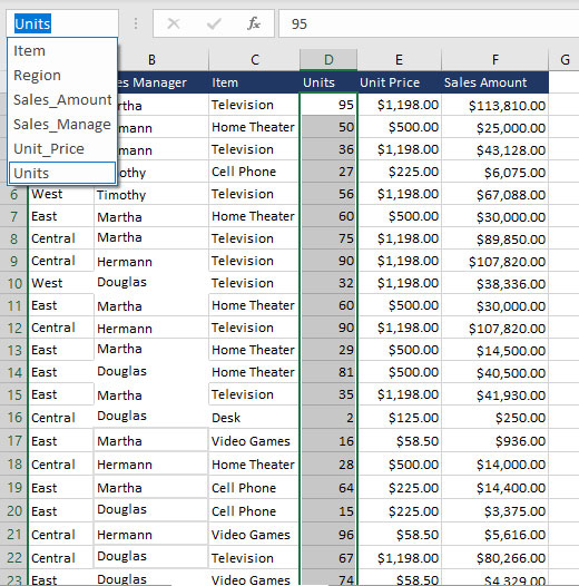
We are going to use a small and simple sales database to perform the functions we introduce in this article. Here is a screenshot of the dataset. We have created named ranges from all columns.

Excel Function for Summarizing Data

In data analysis, it’s often necessary to summarize data based on specific criteria. Excel summarization functions are versatile tools that can be used to quickly and easily identify and summarize data based on user-defined conditions. Here are a few use cases of their practical applications:

• • Summarize Sales by Product Category: Calculate the average/sum/count of sales for different product categories to identify top-selling categories.

• • Identify Best Performance: Identify the salesperson or sales region with the highest average/sum/count (of) sales to recognize top performers.

• • Analyze Customer Spending: Calculate the average/sum/count spending per customer to understand customer purchasing patterns and identify potential upsell or cross-sell opportunities.

• • Monitor Project Costs: Calculate the average/sum cost per project to track project expenses and identify cost-saving opportunities.

• • Compare Performance Across Teams: Calculate the average performance metric for different teams to assess their performance and identify areas for improvement.

Let’s see how Excel summarization functions work in reality.

SUMIF: Summing with a Single Criteria

The SUMIF function in Excel is designed for summing data based on a single criterion. It allows you to add up values in a range that meets a specified condition.

Syntax: =SUMIF(range, criteria, [sum_range])

• • range: Required. The range of cells that you want to be evaluated by criteria.

• • criteria: Required. The condition used to determine which cells to add.

• • [sum_range]: Optional. The actual cells to sum. If omitted, the cells in the range are summed.

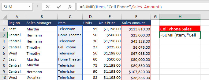
Use Case: Suppose you need to find the total sales for Cell Phones.

Formula: =SUMIF(Item, “Cell Phone”,Sales_Amount )

 

SUMIFS: Summing with Multiple Criteria

The SUMIFS function extends the capability of SUMIF by allowing you to sum data based on multiple criteria. This function is useful when you want to apply conditions simultaneously.

Syntax: =SUMIFS(sum_range, criteria_range1, criteria1, [criteria_range2, criteria2, …])

• • sum_range: The range of cells to sum.

• • criteria_range1: Required. The range to be checked against criteria1.

• • criteria1: Required. The criteria to be met by cells in criteria_range1.

• • criteria_range2, criteria2,… Optional. Additional ranges and their corresponding criteria.

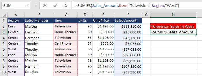
Use Case: We need to find the total sales for Television in the West region.

Formula: =SUMIFS(Sales_Amount,Item,”Television”,Region,”West”)

 

COUNTIF: Counting with a Single Criteria

The COUNTIF function in Excel is used to count the number of cells within a range that meet a specified condition.

Syntax: =COUNTIF(range, criteria)

• • range: Required. The range of cells to count.

• • criteria: Required. The condition used to determine which cells to count.

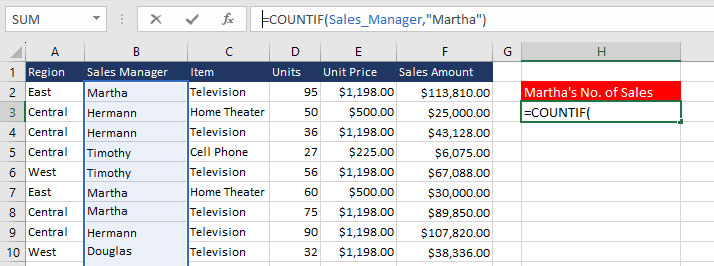
Use Case: Consider we need to count the number of sales for Martha as one of the sales managers.

Formula: =COUNTIF(Sales_Manager,”Martha”)

 

COUNTIFS: Counting with Multiple Criteria

The COUNTIFS function extends the functionality of COUNTIF by allowing you to count data entries based on multiple criteria.

Syntax: =COUNTIFS(criteria_range1, criteria1, [criteria_range2, criteria2, …])

• • criteria_range1: Required. The first range to be checked against criteria1.

• • criteria1: Required. The conditions to be met.

• • criteria_range2, criteria2, …: Optional. Additional ranges and their associated criteria. Up to 127 range/criteria pairs are allowed.

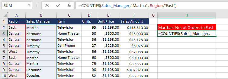
Use Case: Suppose you need to count Martha’s number of sales in East.

Formula: =COUNTIFS(Sales_Manager,”Martha”, Region,”East”)

 

AVERAGEIF: Averaging with a Single Criteria

The AVERAGEIF function in Excel calculates the average of a range of cells that meet a specified condition.

Syntax: =AVERAGEIF(range, criteria, [average_range])

• • range: Required. The range of cells to average.

• • criteria: Required. The condition used to determine which cells to include in the average.

• • average_range: Optional. The actual cells to average. If omitted, the cells in the range are averaged.

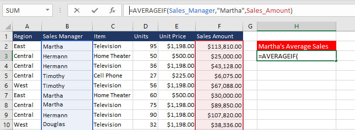
Use Case: Consider you need to find Martha’s average sales.

Formula: =AVERAGEIF(Sales_Manager,”Martha”,Sales_Amount)

 

AVERAGEIFS: Averaging with Multiple Criteria

The AVERAGEIFS function extends the capabilities of AVERAGEIF by allowing you to calculate averages based on multiple criteria.

Syntax: =AVERAGEIFS(average_range, criteria_range1, criteria1, [criteria_range2, criteria2, …])

• • average_range: Required. The range to average.

• • criteria_range1: Required. The ranges to check against the corresponding criteria.

• • criteria1: Required. The conditions to be met.

• • criteria_range2, criteria2, …: Optional. Additional ranges and their associated criteria. Up to 127 range/criteria pairs are allowed.

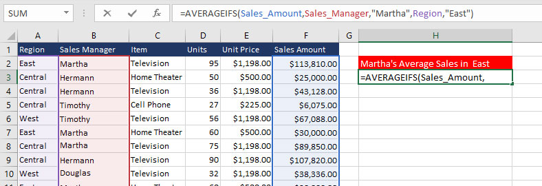
Use Case: Suppose you need to find the average sales for Martha as a sales manager in the East region.

Formula: =AVERAGEIFS(Sales_Amount,Sales_Manager,”Martha”,Region,”East”)

 

 

Excel Lookup Functions

In databases, lookup functions make use of a lookup table to map keys to values. Keys are unique and no value appears more than once. For example, a table connecting author names to their IDs is a lookup table. In this case, lookup functions are used to retrieve an author’s name using their ID. 

In this section, we will investigate Excel’s lookup functions that are frequently used to connect two or more tables that can be used for implementing more sophisticated business logic and data analytics.

CHOOSE

The CHOOSE function works much similarly to the Python list indexing operator. It returns a value from a list of values.

Syntax: CHOOSE(index, value1, [value2], …)

• • index: Required. Specifies the index of the value in the list to be returned.

• • value1: Required. The first element of the list.

• • value2, value3,…: Optional. Additional elements of the list.

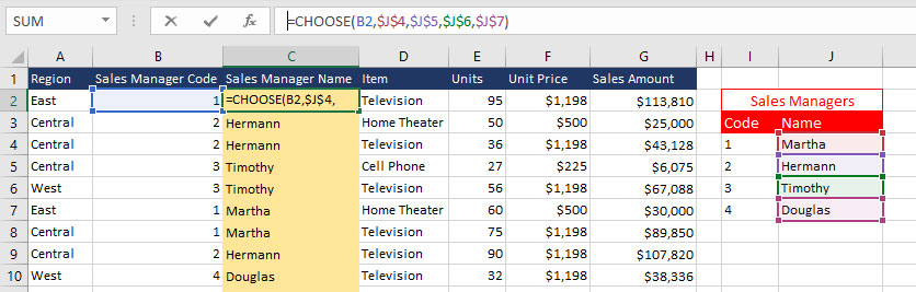
Use Case: In a newer version of our sales dataset, we have a column containing codes of sales managers instead of thei names along with a lookup table. We need to have a column of names instead.

 

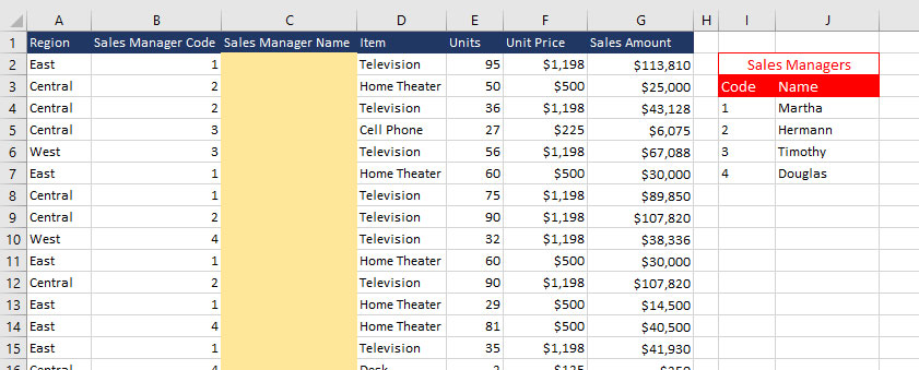
Formula: =CHOOSE(B2,$J$4,$J$5,$J$6,$J$7)

 

VLOOKUP (Vertical Lookup)

VLOOKUP searches for a value in the first column of a table or range and returns a corresponding value from another column.

Syntax: VLOOKUP (lookup_value, lookup_table, col_index, [range_lookup])

• • lookup_value: Required. The value we want to look up.

• • lookup_table: Required. The range of cells in which the VLOOKUP will search for the lookup_value and the return value.

• • col_index: Required. The column number (starting with 1 for the left-most column of table_array) that contains the return value.

• • range_lookup: Optional. Specifies if we want an exact or an approximate match.

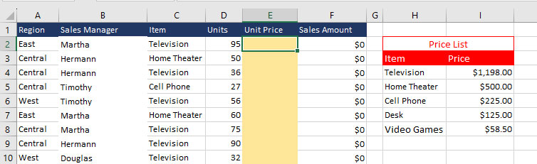
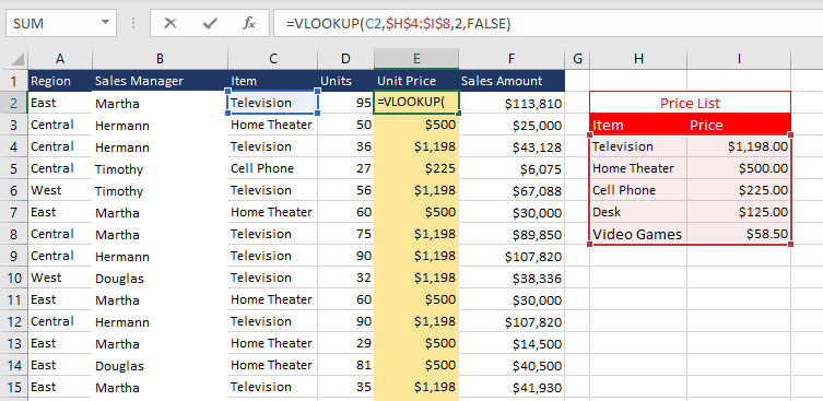
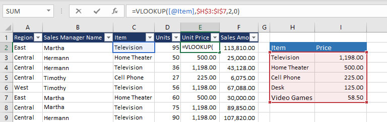
Use Case: Populate the Unit Price column using the vertical price list.

 

Formula: =VLOOKUP(C2,$H$4:$I$8,2,FALSE)

 

We can also use structured referencing in VLOOKUP.

 

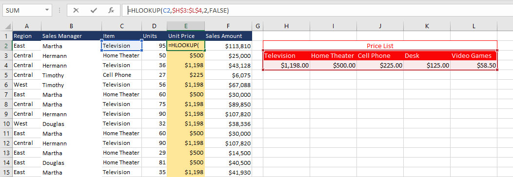
HLOOKUP (Horizontal Lookup)

HLOOKUP is very similar to VLOOKUP except it searches for a value in the first row of a table or range and returns a corresponding value from another row.

Syntax: HLOOKUP (lookup_value, lookup_table, row_index, [range_lookup])

• • lookup_value: Required. The value we want to look up.

• • lookup_table: Required. The range of cells in which the VLOOKUP will search for the lookup_value and the return value.

• • col_index: Required. The column number (starting with 1 for the left-most column of table_array) that contains the return value.

• • range_lookup: Optional. Specifies if we want an exact or an approximate match.

Use Case: Populate the Unit Price column using the horizontal price list.

Formula: =HLOOKUP(C2,$H$3:$L$4,2,FALSE)

 

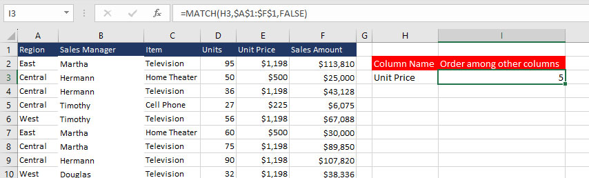
MATCH

MATCH searches for a specified value in a range and returns its relative position.

Syntax: MATCH(lookup_value, lookup_array, [match_type])

• • lookup_value: Required. The value that you want to match in lookup_array.

• • lookup_array: Required. The table or range of cells being searched.

• • match_type: Optional. Specifies how Excel matches lookup_value with values in lookup_array. It can be -1, 0, or 1, for less than, equal to, or greater than matches respectively. The default value is 1.

Use Case: Find the position of a column among other columns.

Formula: =MATCH(H3,A1:F1)

 

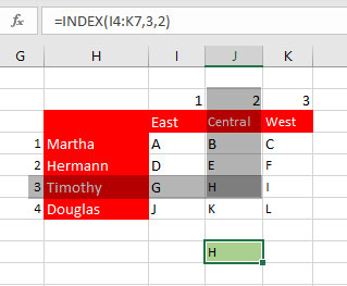
INDEX

Returns the value of a cell in a specified row and column of a table or range. 

Syntax: INDEX(array, row_num, [column_num])

• • array: Required. A range or table of values If contains only one row or column, the corresponding row_num or column_num is optional.

• • row_num: Required. Specifies the row in array from which to return a value. If row_num is not provided, column_num is required.

• • column_num: Optional. Specifies the column in array from which to return a value. If column_num is omitted, row_num is required.

Use Case: Find the category of sales based on Sales Manager and Region. E.g. Find the category of sales for Timothy as sales manager in the Central region.

 

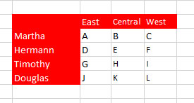
Formula: =INDEX(I4:K7,3,2)

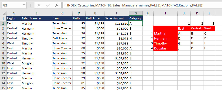
Combining INDEX and MATCH for Dynamic Lookups

INDEX and MATCH are powerful Excel database functions that can be combined to create dynamic data lookup solutions. Let’s explore each function and then see how they can be used together.

Use Case: Add a new column to the data, categorizing sales based on Sales Manager and Region.

 

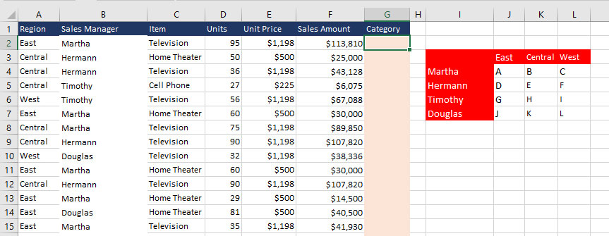
Formula: INDEX(Categories,MATCH(B2,Sales_Managers_names,FALSE),MATCH(A2,Regions,FALSE))

We have used the following named ranges in this formula:

Categories: J5:L7

Sales_Managers_names: I4:I7

Regions: J4:L4

Excel Advanced Database Functions

Excel offers a range of Database Functions that go beyond basic summarization and filtering. These advanced functions, such as DSUM, DCOUNT, and DGET, provide more flexibility and power for analyzing and manipulating data within a database or table.

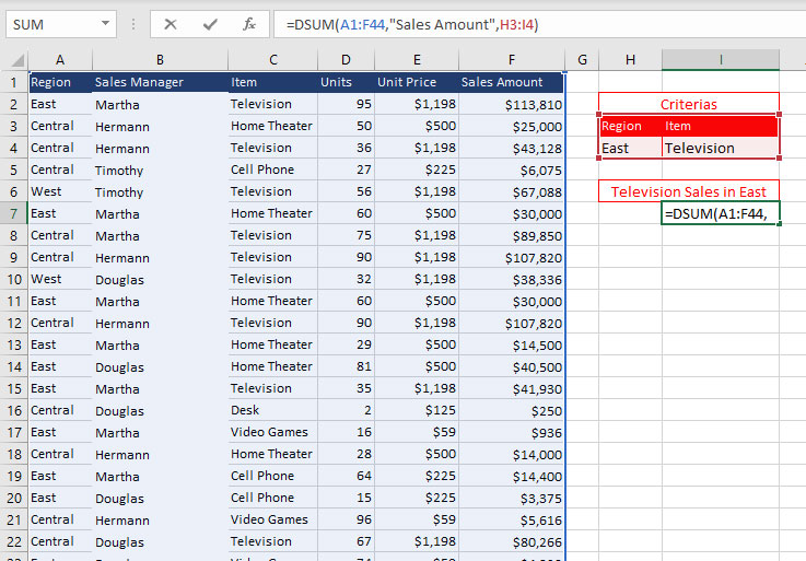
DSUM

The DSUM function in Excel stands for Database Sum. It is an advanced function used for summing up values in a database based on specified conditions. Use DSUM when you need to perform conditional summing on a structured database, allowing for more complex criteria than what is possible with simpler functions like SUMIF or SUMIFS.

Syntax: =DSUM(database, field, criteria_range)

• • database: The range that includes the database table or range.

• • Field: The column or field containing the values to be summed.

• • criteria_range: The range that includes the criteria to be met for summing.

Use Case: Consider you want to find the total sales for the Television in the East region.

Formula: =DSUM(A1:F44,”Sales Amount”,H3:I4)

 

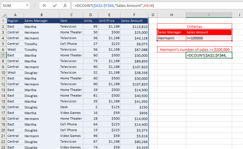
DCOUNT

The DCOUNT function in Excel, short for Database Count, is used to count the number of entries in a database that meet specified criteria, providing a more dynamic and structured approach than COUNTIF or COUNTIFS.

Syntax: =DCOUNT(database, field, criteria_range)

• • database: The range that includes the database table or range.

• • Field: The column or field containing the values to be counted.

• • criteria_range: The range that includes the criteria to be met for counting.

Use Case: You want to count the number of Hermann’s sales that are above $100,000.

Formula: =DCOUNT(A1:F44,”Sales Amount”,H3:I4)

 

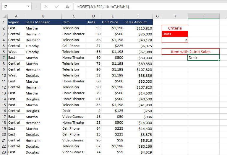
DGET Function

The DGET function, or Database Get, is used to extract a single value from a database based on specified conditions, providing a more precise result than VLOOKUP or INDEX/MATCH.

Syntax: =DGET(database, field, criteria_range)

• • database: The range that includes the database table or range.

• • Field: The column or field containing the value to be extracted.

• • criteria_range: The range that includes the criteria to be met for extraction.

Use Case: You need to extract the Item with 2 Unit Sales.

Formula: =DGET(A1:F44,”Item”,H3:H4)

Excel External Data Sources

Excel provides seamless integration with various external data sources. This allows accessing and manipulating data from files (Excel Workbooks, Text/CSV, XML, JSON), databases (Access, SQL Server, Oracle, IBM Db2, PostgreSQL), Azure, Online Services (MS SharePoint, MS Dynamics), and other services (Microsoft Exchange, web services). This eliminates the need to copy and paste data from disparate sources manually. In this section, we will show how to use this functionality using real-world examples.

Connecting to SQL Databases

To connect Excel to an SQL database, follow these steps:

1. 1. Open the Excel workbook where you want to import data.

1. 1. Go to Data -> Get & Transform Data -> Get Data -> From Database and select From SQL Server.

1. 1. In the SQL Server database wizard, specify the connection details, including the server name, database name, and authentication credentials.

1. 1. Once the connection is established, you can select the tables or views you want to import.

Connecting to Web Services

To connect Excel to a web service follow these steps:

1. 1. Go to Data -> Get & Transform Data -> From Other Sources and select From Web.

1. 1. In the Connect to Web dialog box, provide the URL of the web service and the desired data source.

Important Note: 

3. 3. Excel will attempt to parse the web service data and present it as a connection.     Once the connection is established, you can select the tables or data structures you want to import.

When you click on that it will automatically go to your browser home page and if there were scripts on that page you might get some errors. So, just click no until the errors go away. Then come into the address bar and paste in your URL and click go. 

And again if there are errors on the web page you will get these errors popping up. So we’re just going to click No until they go away. Now to link to data on the web that data must be stored in a table. 

But you’ll find that generally things like currency exchange rates price lists are in tables and you can spot the tables because they’ve got little yellow arrows next to them. And to select one click on the yellow arrow and then click Import and say okay. And in a moment that live data will be loaded into your workbook. 

Now it won’t automatically refresh but you can right-click on the data at any point and choose the refresh option or if you want to you can come to the data range properties.

 And you can specify, I’ll just move that up, you can specify that you wanted to automatically refresh every hour or every five minutes, but bear in mind that that may impact the performance of your workbook. We’re going to leave it at this and say okay. So here’s our data. 

Using Database Functions to Manipulate External Data

Once you have connected Excel to an external data source, you can utilize database functions to manipulate and analyze the imported data. For instance, you can use the SUM, AVG, and COUNT functions to aggregate data or use the Filter and PivotTables to perform advanced data analysis.

Optimizing Database Functions

Database functions in Excel are powerful tools for manipulating and analyzing data. However, they can also be computationally expensive, especially when dealing with large datasets. To maximize the efficiency and performance of these functions, follow these optimization tips:

Use Array Formulas Prudently

Array formulas are efficient for performing operations on multiple cells simultaneously. However, they can also consume significant processing power. Use array formulas only when it’s necessary to handle multiple cells at once. For single-cell operations, consider using standard formulas.

Minimize Used Range

Excel recalculates formulas based on the used range, which is the area of cells that contain formulas and are visible in the worksheet. To optimize performance, minimize the used range by hiding or protecting unused cells. This will prevent unnecessary recalculations and improve overall worksheet speed.

Utilize Named Ranges

Named ranges provide a way to assign descriptive names to ranges of cells. This can make formulas more readable and easier to modify. Additionally, named ranges can help reduce typing and improve code consistency.

Employ Index and Match for Dynamic Lookups

The INDEX and MATCH functions are more versatile and efficient than traditional lookup functions like VLOOKUP or HLOOKUP for dynamic lookups. They can handle multiple lookup criteria and approximate matches, making them suitable for complex lookup scenarios.

Avoid Circular References

Circular references occur when a formula refers to itself or other formulas that directly or indirectly refer to it. While they can be useful for creating self-updating calculations, they can also lead to infinite loops and performance issues. Avoid circular references unless they are necessary.

Optimize PivotTables

PivotTables are powerful tools for summarizing and analyzing data. However, large PivotTables with complex calculations can become sluggish. Optimize PivotTables by minimizing the number of fields, limiting calculations, and avoiding unnecessary data aggregation.

Consider VBA Macros

For repetitive tasks or complex data manipulation, consider using VBA macros. VBA macros can automate repetitive processes and improve the efficiency of data analysis. However, use macros judiciously to avoid introducing unnecessary complexity and performance overhead.

Best Practices for Efficient Database Function Usage

• • Structure Data Efficiently: Organize data consistently and logically to facilitate easy manipulation and analysis.

• • Avoid Data Duplication: Minimize data redundancy by consolidating similar data into a single location. This reduces the need for repeated lookups and calculations.

• • Standardize Data Formats: Ensure consistent data formats across different datasets to avoid errors during data manipulation and analysis.

• • Regularly Review and Optimize Formulas: Periodically review formulas to identify areas for optimization and potential performance improvements.

• • Utilize Data Validation: Implement data validation rules to prevent incorrect data entry and ensure data integrity.

• • Implement Data Governance: Establish and enforce data governance principles to maintain data consistency, accuracy, and security.

• • Leverage Excel’s Automation Tools: Utilize Excel’s automation tools, such as macros and scheduled tasks, to automate repetitive tasks and streamline data processes.

• • Monitor Performance and Identify Bottlenecks: Regularly monitor and analyze worksheet performance to identify potential bottlenecks and optimize performance.

• • Consider Data Warehousing Solutions: For large-scale data analysis and reporting, consider implementing a data warehousing solution to store, manage, and analyze large datasets efficiently.

 

Resources for Further Learning

Here are some recommended resources for readers who want to deepen their knowledge of Excel database functions:

Books

• • Microsoft Excel 2016 Bible by John Walkenbach – This comprehensive guide covers a wide range of Excel topics, including database functions. It’s suitable for both beginners and advanced users.

• • Excel 2016 Power Programming with VBA by Michael Alexander and Richard Kusleika – While focusing on VBA programming, this book covers advanced Excel functions, including database-related tasks.

• • Power Query for Power BI and Excel by Chris Webb – Power Query is a powerful tool for data transformation in Excel. This book is ideal for those interested in enhancing their skills in working with external data.

Online Tutorials

• • Excelisfun – This website provides a wealth of free Excel tutorials, including tutorials on database functions.

• • Lynda.com – Lynda.com offers a subscription-based service with a wide variety of Excel training courses, including courses on database functions.

• • ExcelJet – This website provides a variety of Excel resources, including tutorials on database functions.

Courses

• • Excel for Business Professionals by Coursera; University of Michigan – This course covers a wide range of Excel topics, including database functions.

• • Excel and Data Analysis by edX; University of Virginia – This course covers a variety of Excel topics, including database functions, with a focus on data analysis.

• • Excel Masterclass by Udemy – This comprehensive course covers all aspects of Excel, including database functions, in a thorough and well-structured way.

 

Conclusion

As you navigate the dynamic world of data analysis, Excel stands as a powerful tool, but its true potential lies in its versatile database functions. This article tried to help you connect Excel to external data sources, model the data in Excel using relationships, and then utilize Excel database functions to analyze the data. 

With this newfound mastery, you’ll be able to extract meaningful insights from complex datasets, transforming raw numbers into actionable knowledge. You’ll be able to query, filter, and analyze data with ease, enabling you to make informed decisions that drive success. Embrace the power of Excel’s database functions and elevate your data management skills to new heights.

 

FAQ