How To Use Solver In Excel

Excel solver is a built-in tool by Excel, which is used to solve linear program problems. You can actually use it to solve both linear and non-linear problems.

It’s a handy tool for making decisions regarding optimization problems. Optimization of these decisions will surely help you to maximize your profits.

Let’s take a look at how to use Excel solver for solving linear problems in this Excel solver tutorial:

First, you will have to enable Solver as a feature to Excel as it’s not enabled by default.

1. Click on File and navigate to the Options tab
2. In the options window, click on Add-ins
3. With the Excel Add-ins options selected from the dropdown menu, click on Go.

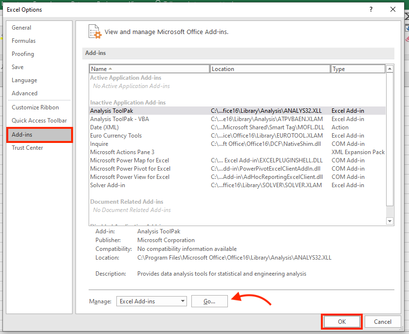
4. In the new window, select Solver Add-in and then click OK. 

Note: you might receive a message that Excel solver add-ins are not installed on your computer. Click on Install to do so. 

After following these steps, Solver should appear under the Data tab in the Analysis group. 

Before you can start using Solver, you have to have your formula ready. 

In our example, we’re going to look at a carpentry shop that is looking to provide services, but in order to do so, it needs to purchase new equipment that costs $40,000 which is going to be paid in the form installments over 12 months.

The goal is to reduce – as much as possible – the cost per service provided by the carpentry shop during those 12 months.

So we created this using the numbers:

Cost of new equipment $40,000

Estimated No. of clients per month 50

Cost per service ?

No. of months to pay =B3/(B4*B5) = 12

Now, let’s see how we can optimize this problem and find a solution using Solver in Excel.

1. First, go to the Data tab, and under the Analysis Group click on Solver.
2. In the new window, you have to define 3 components in order to solve the problem:
   1. Objective Cell
   2. Variable Cell
   3. Constraints

What happens is that Excel tries to find the optimal solution for the “objective cell” by changing the data in the variable cell and trying to maximize or minimize the value of the objective cell. It does so by taking into account the constraints or limitations that we have defined in the appropriate cell.

Objective cell

This is the cell that contains the formula which tells us the goal and our objective for the problem. Is our aim to maximize, minimize or reach a specific value?

In the example we mentioned above, this cell is B7, which contains the formula =B3/(B4*B5) that results in number 12 as value. 

Variable Cell

This cell contains the variable data that will be changed by the Solver to achieve the objective that we explained above. 

In the example we first mentioned, we have two variable cells:

• Estimated No of clients (cell B4) which should be equal to or less than 50
• Cost per service (cell B5) which is the value we want the Solver to calculate

Constraints

Constraints are the limitations that we can put on the problems. These are the conditions that we specify which have to be met before an optimal solution is achieved.  

In order to set a constraint, follow these steps:

• Click on the Add button next to the Subject to Constraints box
• In the new window, enter a constraint
• Click on Add
• You can keep adding other constraints
• Click OK to finish

There are different relationships that you can define between the reference cell and the constraint. 

If you want to delete a constraint, follow these steps:

• Open the Solver Parameters window and click on the constraint
• If you’re going to edit it, click change and then make the changes you need
• If you would like to delete it, click on the delete button

Solving the problem

After following all these steps and finishing the required configuration, you can solve the problem. In order to do so, click on the Solve button at the bottom of the Solver Parameters windows, which we used before.

Solving the problem depends on the amount of data and the parameters which you previously configured. Because of the resource usage of the calculations, the solving could take a few seconds, minutes or even hours.

After the calculations and the processing has finished, the Solver will display the Results window. Select “keep Solver solution” and then click OK.

The results will be displayed in the worksheet.

In our example, in cell B5, we will see 66.67 dollars, which should be the minimum cost per service you will charge in order to pay for the equipment in the 12 months set beforehand.

Now let’s take a look at some Excel solver examples.

We are going to look at a simple transportation problem that is solved by a linear programming equation. This is a simplified version of a very complex equation that is solved every day by major companies around the world. 

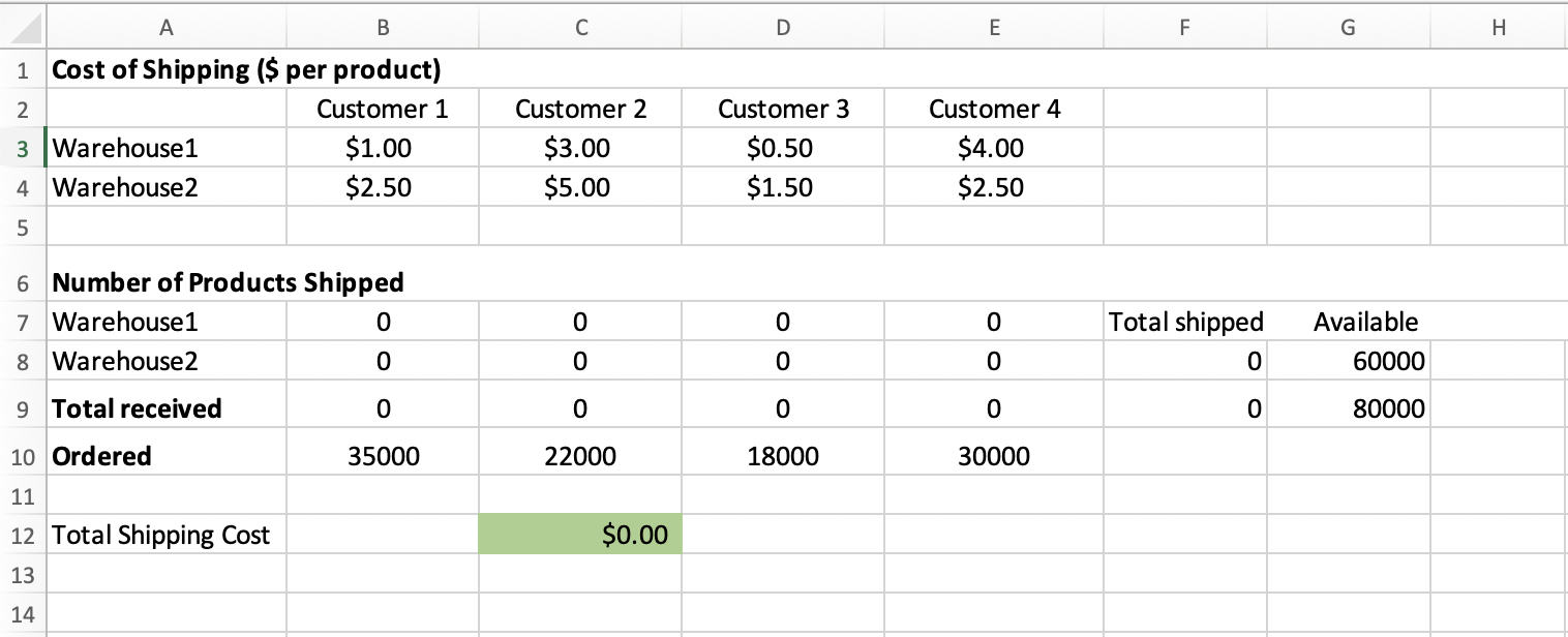
This is the problem: we want to minimize the cost of shipment products from two warehouses to four customers. The warehouses have limited supply, and the customers have limited demand.

Our goal is to limit shipment costs without going over our demand and supply limits (constraints).

The data

Here is what our data looks like:

Setting up the model

In order to create the model, we have to answer these questions:

1. What decision do we have to make to reach the optimal quantities delivered from each warehouse to each customer? 
2. What are our constraints or limitations? The supply and demand numbers are the constraints.
3. What is the goal? Our goal is to reduce the cost of shipping and get to the minimum point. 

The next step is to calculate the total number of shipped products from the warehouse and the total number of products received by the customer. A SUM formula can do this.

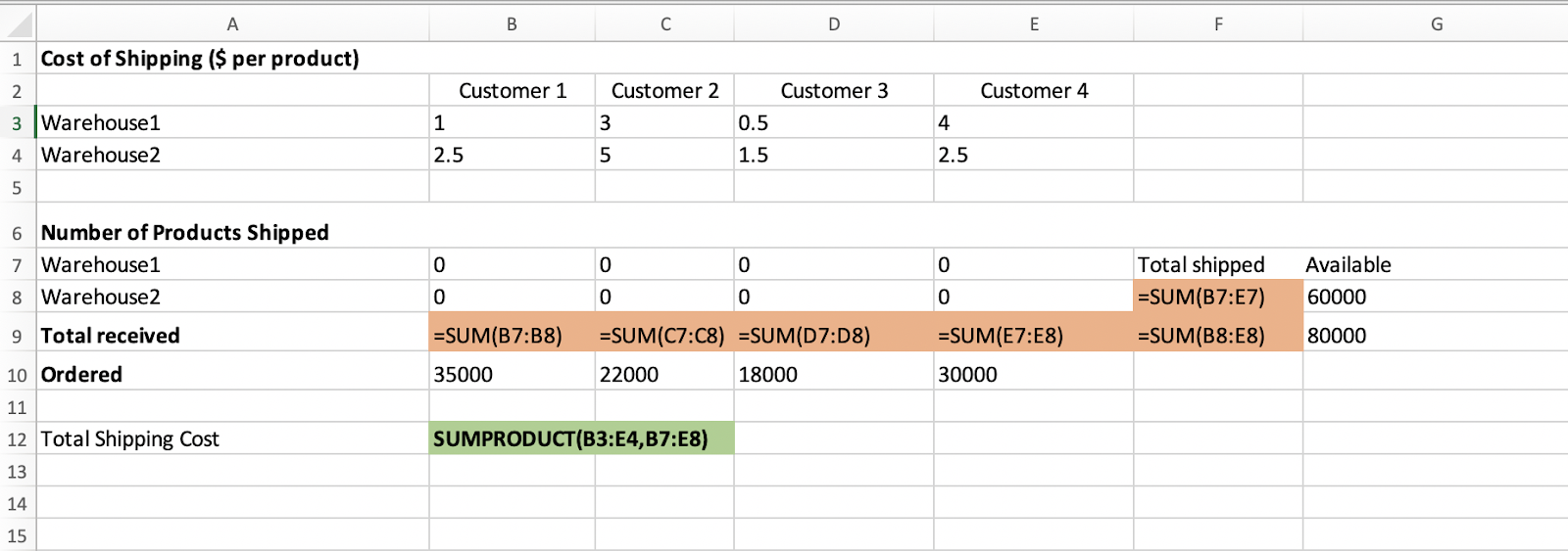
In order to better understand the example, we’re going to name the ranges as so:

Range name	Cells	Solver parameter
Products_shipped	B7:E8	Variable cells
Available	I7:I8	Constraint
Total_shipped	G7:G8	Constraint
Ordered	B10:E10	Constraint
Total_received	B9:E9	Constraint
Shipping_cost	C12	Objective

The last step is to do these configurations in the Solver program as before.

• The objective is the Shipping cost which should be set to minimum
• The variable cells the Products shipped
• And the Constraints are according to  the table above.

In the end, click the solve button like the example we followed before. The solution will be calculated and entered into the worksheet.

By this Excel solver tutorial, we would use the Solver to make better decisions regarding optimization problems.