Freezing Rows And Columns In Excel

While working with large data sets in Excel, you’re usually forced to scroll down a lot, which will take the title of the columns and rows out of your sight. 

In situations like this, you can use the Excel Freeze Panes feature for keeping certain rows or columns in the view. By doing this, you will always have the selected rows and columns in view regardless of how far down you scroll. 

Accessing the Options for Excel Freeze Panes

Follow these steps:

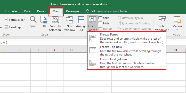
• Click on the View tab
• Click on the Freeze Panes menu
• You will see three options:
  • Freeze Panes: This allows you to freeze select rows or columns
  • Freeze top row: This just freezes the first top row of the excel sheet.
  • Freeze the first column: By choosing this option, the first left column will be frozen.

You can use these options for freezing rows or columns (or both) in Excel panels.

Let’s see how we can use these tools for freezing rows or columns in Excel while working with large data sets. 

Enhance your business efficiency with our specialized Macro Development Services, tailored to automate and streamline your operations for maximum productivity

Freezing Rows in Excel

If you’re working with a large dataset and your columns have headers, as soon as you start scrolling down, the titles of the columns will move out of your sight. Like the example below:

In cases like these, it’s good practice to freeze the title rows, so they’re always visible.

In this part we’re going to learn:

• How to freeze the top row
• How to freeze more than one row
• How to unfreeze rows

Freezing the Top Row in Excel

We’re going to the first row in your dataset:

• Click on the View tab
• Click on the Freeze Panes menu
• Click on the Freeze Top Rows option
• This action will freeze the first row. Now you can see a visible grey line under the frozen row.

Now, if you scroll down, the frozen line will not move and will always stay in view. This is what you will see:

Freezing/Locking More than One Row in Excel

In some cases, you might need to freeze a few rows. Let’s see how to do that:

• Select the furthest cell on the left side which is below the title row
• Click on the View tab
• Click on the Freeze Panes menu
• Select the Freeze Panes option

This action will freeze all the rows above the selected cell. A grey line will appear below the frozen cells. 

Now when you scroll down, all the frozen rows will be kept in view.

Unfreezing Rows

Follow these steps for unfreezing rows:

• Click on the View tab
• Click on the Freeze Panes menu
• Select the Unfreeze Panes option

Freezing Columns

If you’re working on a table that has titles under one column, you might have to freeze the column because it will move out of sight if you have to scroll sideways. An example is shown in the video below:

In this case, you can freeze the first column on the left to keep it in sight.

We’re going to learn how to:

• Freeze the far left column
• Freeze more than one column
• Unfreeze columns

Freezing/Locking the Far Left Column

We’re going to look at the steps on freezing the far left column in Excel:

• Click on the View tab
• Click on the Freeze Panes menu
• Select the Freeze First Column option

This action will freeze the furthest left column. You can see a grey line appearing next to it and separating it from other columns. 

Now while scrolling sideways, the frozen column will always stay in view. Example blew:

Some hints:

• After freezing a column, you cannot use Ctrl+Z to undo the action. You have to use the Unfreeze option from the Freeze Panes menu.
• If you place a column to the left of the already frozen column, the new column will become frozen as well. 

Freezing/Locking More than One Column in Excel

If you have more than one column that contains titles in your worksheet, you might want to freeze them all. Follow the steps below:

• Select the highest cell on the column to the right of the title column
• Click on the View tab
• Click on the Freeze Panes menu
• Click on the Freeze Panes option

This will freeze the columns to the left of the selected cell. You will see a grey line separating the frozen columns from the others. 

Now while you scroll to the right, all the frozen columns will stay visible as in the example below:

Unfreezing Columns

Follow these steps to unfreeze columns:

• Click on the View tab
• Click on the Freeze Panes menu
• Select the Unfreeze Panes option. 

Boost your productivity by getting a free consultation from Excel experts, and discover tailored solutions to optimize your data management and analysis.

Freezing Rows and Columns 

In most cases, you’re likely to have both columns and rows that contain the title. That’s why you’re going to need to freeze both columns and rows.

Follow the steps:

• Select the first cell after the rows and columns which you’d like to freeze. For example, If you want to freeze two rows (rows 1 and 2) and two columns, (A and B) select cell C3
• Click on the View tab
• Click on the Freeze Panes menu
• Click on the Freeze Panes option

This action will freeze columns to the left and the rows above the selected cell. (C3). A grey line will separate the frozen rows and columns from the rest. 

Now when you scroll down or to the side, you can see the frozen rows and columns. An example is shown below:

You can unfreeze rows and columns at the same time:

• Click on the View tab
• Click on the Freeze Panes menu
• Select the Unfreeze Panes option

Some notes:

• One of the other uses of freezing in Excel – other than when working with large datasets – is dashboards. When using a dashboard, you might want to freeze some rows or columns, so the user can always have the dash in view.
• A good practice while working with large datasets is transforming it into Excel tables. By default, Excel tables will always keep the title rows or columns in the view, without having to freeze them manually.