How Can The Conditional Format Help You in Excel?

If you have created an important, but lengthy Excel sheet, containing lots of information, it might be hard to find the data you want. For example, you may need to analyze your sales and find the values that are higher or less than a certain amount. That’s only one of the scenarios that conditional formatting in Excel can solve. Therefore, learning what it is and how it works can be of considerable help when working with Excel.

Conditional Formatting in Excel: Highlight Cells Rules

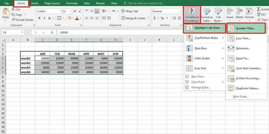
You can use conditional formatting in Excel to highlight numbers that are higher, less than a number, or even between two numbers. It’s so simple. Just start by choosing the table or columns that you want to find your preferred values in.

Highlight numbers that are higher than X 

 In our example, we want to find values that are higher than 15000. 

1. From the “Home” tab Click on “Conditional Formatting” in the “Styles” group. 
2. When the menu opens, click on “Highlight Cells Rules” and choose “Greater Than”.

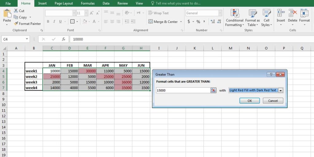
3. Now you can choose the value you want to analyze your data based on it. In our example, we have chosen 15000. 
4. We also want to highlight the numbers in red, which you can change from the drop-down menu in front of the number field. 
5. You can see that all the cells that have values greater than 15000 turn red. 

Highlight numbers that are less than X 

Just like the previous example, you can highlight values that are less than a special number. In our example, we want to find values that are less than 10000. 

1. Follow steps one and two. This time, choose “Less than”. 

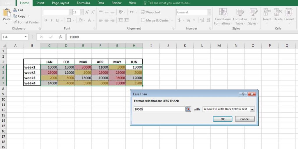
Fill the field with your preferred value and choose the highlight formatting from the drop-down menu. We have chosen a different color for numbers that are less than 10000. However, the changes depend on your preferences.

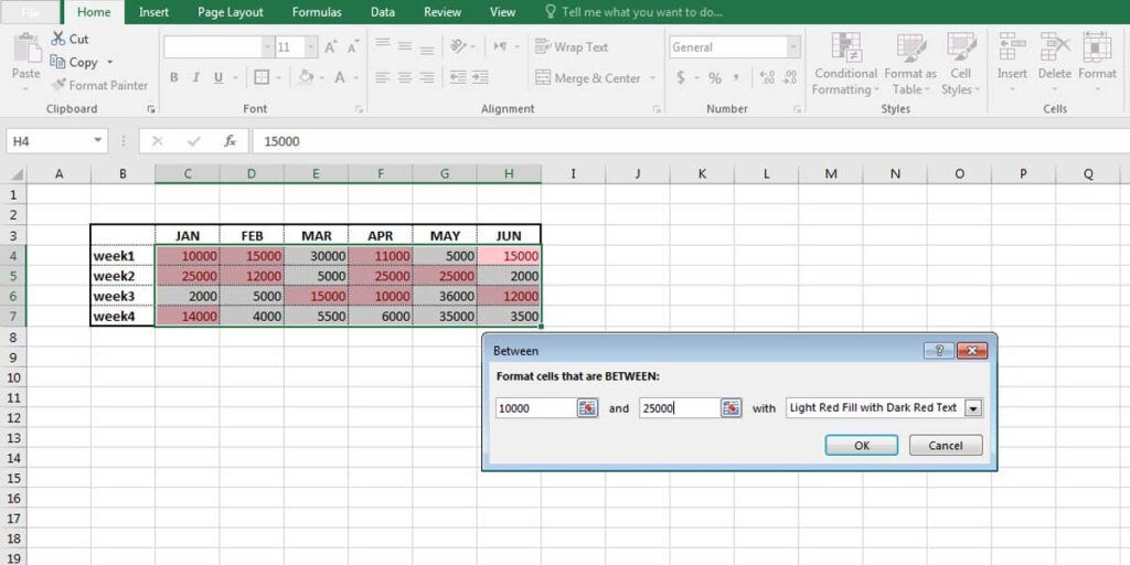
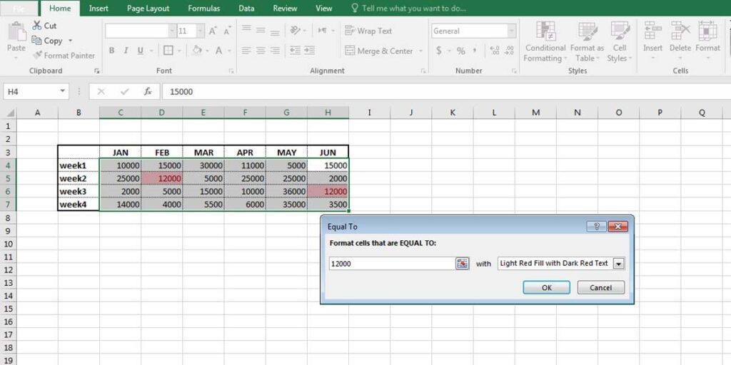
Just like both examples, you can find numbers that are between two other values, or numbers that are equal to the value you chose. All you have to do is follow the steps above and choose the other two relevant functions, called ‘Between’ and ‘Equal To’.

Conditional Formatting in Excel: Top/Bottom Rules 

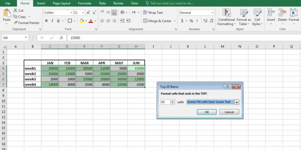
Top 10 items/ Bottom 10 items 

As we mentioned before, Conditional Formatting helps you highlight important values visually, using color, icons and bars. This part of the Conditional Formatting menu is based on Excel calculations. It’s used when you want to know the best and worst values. For instance, if you want to know the top 10 sales you had, you can choose “Top 10 items” from the list. Excel checks the cells and finds the highest values. However, you can change the number of items you want to show to less or more than 10.

The steps are the same for finding the minimum values on the form. This time you need to choose “Bottom 10 items”.

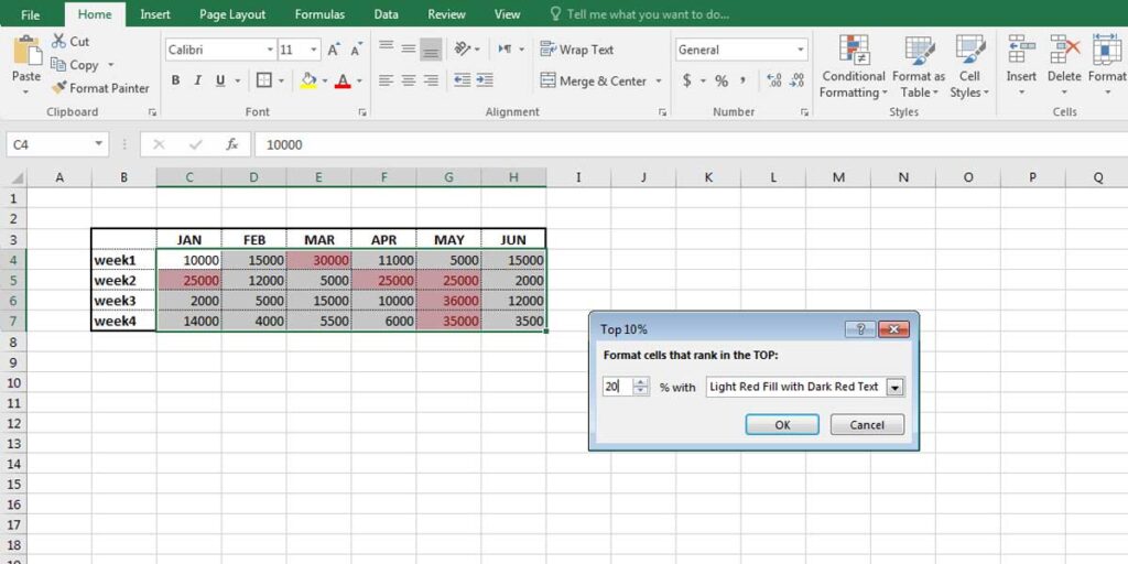
Top 10%/ Bottom 10%

Sometimes you may want to find the highest and the least values based on a percentage. You can easily find the function in the Conditional Formatting list.

You can find two functions under the Top/Bottom Rules list: one for top 10% and the other for bottom 10%. Choose one based on your preferences. 

By default, Excel shows you the top 10% of the selected items. You can also change that to any other percentage you want.

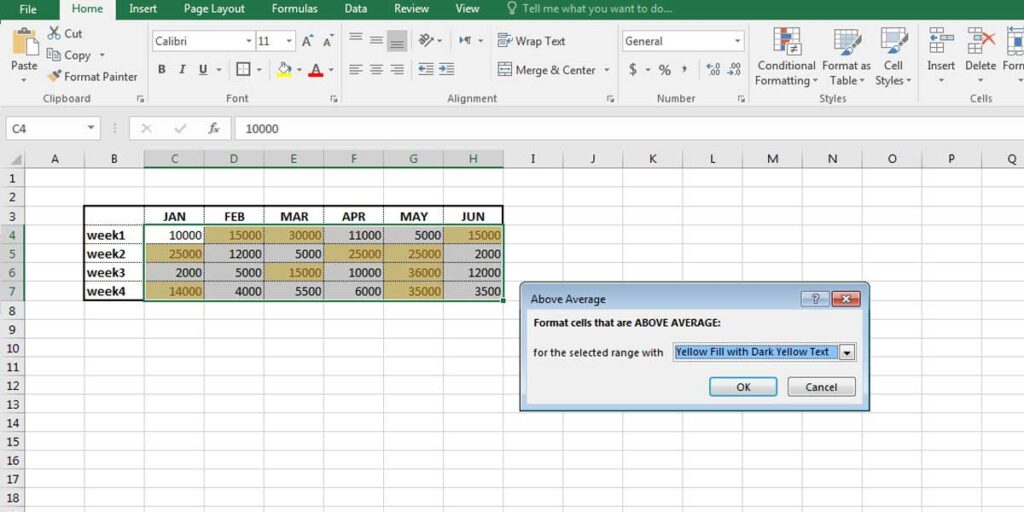
Above and Below Average  in excel

Similarly, aside from calculating average in excel, you can find the figures below or above average using this option. 

1. You just need to select the cells you want to analyze. 
2. Go to the “Conditional Formatting” menu, find “Above Average” or “Below Average” – based on your preferences- under Top/Bottom Rules. The result will be as follows. 

Above Average: Excel finds the average of the selected values and shows the cells containing numbers that are higher than the average.

Below Average: Excel highlights the cells that contain numbers that are less than the average.

You can also choose the highlighting format from the drop-down menu. 

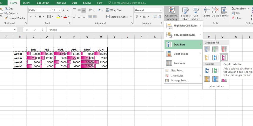
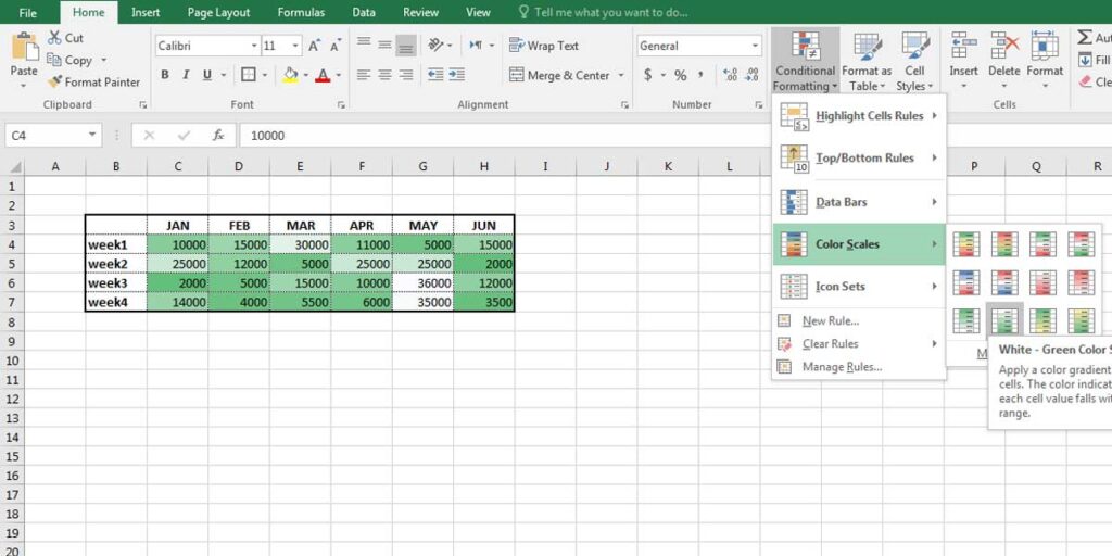
Changing the Highlight Appearance 

The main feature in Conditional Formatting is changing the appearance based on the conditions you specify. This is part of the data visualization technique, which can help you analyze data and detect crucial issues. 

Perhaps, you intend to show the highest to the lowest values on a form or a selection.  You have these options:

Data Bars: You can highlight the values by data bars. The lowest value has the smallest bar, and the highest will have the fullest bar. It is also possible to choose a solid color or gradient for these bars. 

Color Scales: This is another form of showing the highest and the lowest numbers in a form. This function dedicates a unique color to each number. 

Icon Sets: It’s also possible to format each cell with an icon, such as up and down icons, shape, and ratings.

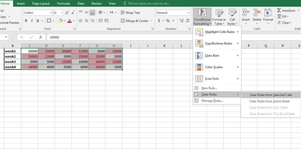
Clearing Conditional Formatting Rules in Excel 

There are times when you have conditional formatting on a worksheet, and you wish to remove it. Excel has provided the Clear Conditional Formatting option for such circumstances.

1. Select the cells you want to clear the rules from. 
2. Under the “Conditional Formatting” menu, go to “Clear Rules” and click on the “Clear Rules from the selected cells”. 

Manage Rules | Excel Conditional Formatting Rules Manager

Remember, you can easily create, delete, edit and view all conditional formatting rules. To be able to manage such data manipulation, you can use the Conditional Formatting Rule Manager Dialogue box. 

For instance, select “Manage Rules” under the “Conditional Formatting” menu to change the highlight colors and appearance or any other function.

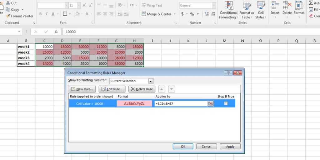
You can either add new rules, edit the current rules, or delete any of them. 

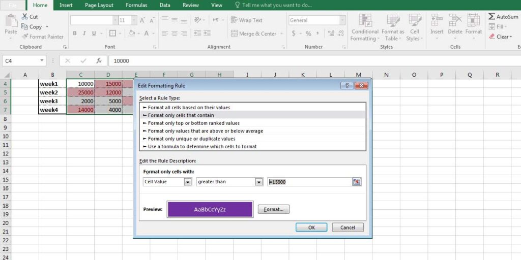
1. Select the rule and click on “Edit Rule”. 
2. A new window opens where you can edit and change anything about the selected rule. In our example, we decided to change the color of the highlight and also edit the rule and show values that are greater than 15000. The result is as follow: 

Conditional Formatting with Formulas

This method embraces a wide range of functions, which means you can write any formula and highlight its results. You can find an example for this in the article about comparing two columns in excel. 

1. Go to “Home” and click on “Conditional Formatting”. 
2. Click on “New Rule” and select “Use a formula to determine which cells to format”. 
3. Write the formula you want and change the formatting type as you prefer. 
4. Click OK and see the result. 

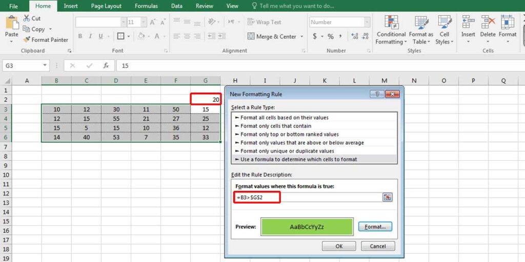
In our example, we wrote a formula that checks all the cells to see if they are higher than G2. As a result, whenever we write another number in G2, the highlights will change without any need to change the formula. 

IFS Function

The IFS function is another way of writing a conditional formula, which lets you have several logical conditions and gives you a result in the cell in which you have written the formula. This method is a more advanced method which we have completely explained in the IFS function method. 

Bottom Line 

The Conditional Format in Excel is highly functional. You can visually analyze your data in a few steps, while having a wide variety of formats to choose from. You can do simple tasks such as finding the values you are looking for, by writing your own formula or even applying conditional formatting to a PivotTable report.