How To Calculate Average In Excel

The average is a typical exhibition of a data set, which is provided in the Excel spreadsheet in 4 functions for various situations. In this tutorial, we’re going to learn how to use these functions in Excel. 

In this blog (and many other articles) average and mean are used interchangeably. 

In mathematics, the average is the same as “arithmetic mean” or simply mean. To be more precise, it has to be stated that “mean” has several definitions, one of which i.e. arithmetic mean is equal to average. Geometric and harmonic mean are examples of different mean concepts and definitions.

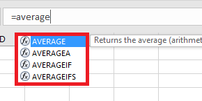
According to picture 1, the average functions include:

AVERAGE 

Which is used to calculate the arithmetic mean for a group of numbers.

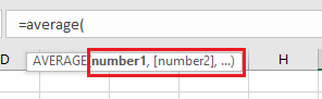
The Set of data, which is one or more numeric values, is the number in the syntax of the function.

There are more ways to calculate the average:

1. Use the AVERAGE function (according to video 1):

1. Enter the AVERAGE function in an empty cell.
2. Select your data as a range.
3. Press Enter.

2. Use the SUM function and divide by the COUNT function according to video 2:

1. Enter the SUM function in an empty cell.
2. Select your data as a range.
3. Divide by the COUNT function.
4. Select your data as range, again.
5. Press Enter.

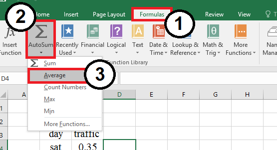
3.  Add a quick calculation to your worksheet, automatically, such as the AVERAGE.

1. Select an empty cell.
2. Click on the FORMULAS tab.
3. Click on the AUTOSUM.
4. Select the AVERAGE from the list.
5. Highlight your target data.
6. Press Enter.

 

4.  Use the QUICK ANALYSIS TOOL (Ctrl+Q) to quickly and easily analyze your data with some of Excel’s most useful tools, like the AVERAGE (according to video 3.)

1. Select your data.
2. Click on the QUICK ANALYSIS TOOL icon (at the bottom of the data.) or press Ctrl+Q.
3. Select the TOTALS tab from the toolbar.
4. Click on the AVERAGE.

5.  Use the INSERT FUNCTION (Shift+F3), and pick the AVERAGE function from the STATISTICAL category (according to video 4.)

1. Select an empty cell.
2. Click on the FORMULAS from the ribbon.
3. Click on the INSERT FUNCTION.
4. Search the “AVERAGE” in the “search for a function” box or select the “Statistical” category from the “select the category” menu and select the AVERAGE in the “select a function” list. Then press OK.
5. Enter your data (number 1, number 2, etc.) and press OK.

The AVERAGE relinquishes empty cells and cells that contain text (it doesn’t ignore zero values.)

You can calculate the average in excel 2007 and later, for up to 225 number arguments.

 

 

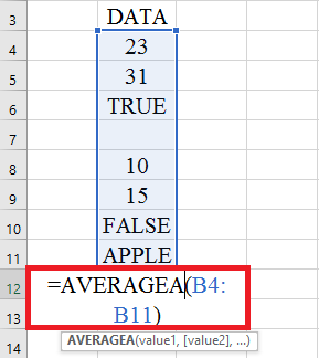
AVERAGEA

This function works like the AVERAGE. However, if you have cells that contain text or the logical value FALSE, the AVERAGE will assess it as zero. Also, the logical value TRUE is assessed as 1.

There is another way to calculate the AVERAGEA function; using the INSERT FUNCTION (according to video 5.)

1. Select an empty cell.
2. Click on the FORMULAS from the toolbar.
3. Click on the INSERT FUNCTION.
4. Search for the “AVERAGEA” in the “search for a function” box or select the “Statistical” category from the “select the category” menu, and select the AVERAGEA in the “select a function” list. Then press OK.
5. Enter your data (value 1, value 2, etc.) and press OK.

AVERAGEIF

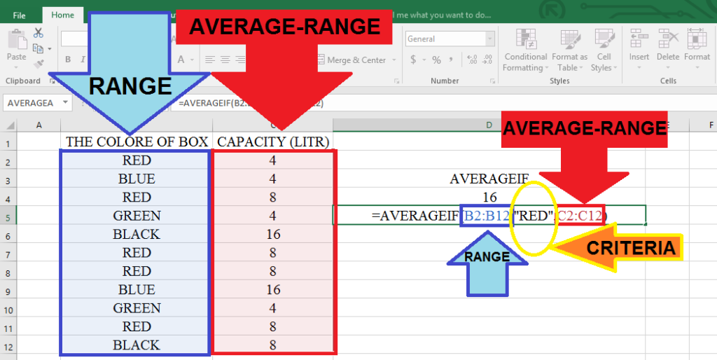
This Excel function distinguishes the values in a range of cells and finds the average for them that meet the defined criteria. 

AVERAGEIF is used when you need to calculate the average of a data set with only one criteria in mind. For example, the average of numbers equal to or more than 10 or data related to a specific category. If you have more than one criterion, you will have to use the AVERAGEIFS function.

1. Select an empty cell.
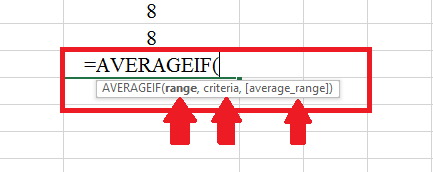
2. Enter “=AVERAGEIF” and press Enter.
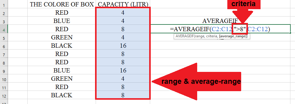
3. Define the “range.” (Defining the range depends on your criteria. Pay attention to picture 6 & 7)
4. Define the “criteria.” (Enter your criteria among “ ”)
5. Define the “average-range.”
6. Press Enter.

Use the INSERT FUNCTION on the FORMULAS tab to calculate the AVERAGEIF. Follow these steps or watch video 6:

1. Select an empty cell.
2. Go to the FORMULAS tab and select the INSERT FUNCTION.
3. Search for the AVERAGEIF or select the STATISTICAL category.
4. Select the AVERAGEIF from the menu and press OK.
5. Enter the RANGE, the CRITERIA, and the AVERAGE-RANGE. Then press OK.

The point is the AVERAGE-RANGE must include a numerical value. If your AVERAGE-RANGE contains text value or a blank cell, the result returns the #DIV/0! error.

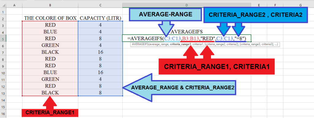
AVERAGEIFS

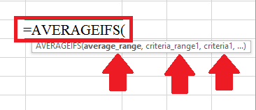
A multiplex peer of the AVERAGEIF function is the AVERAGEIFS. You can specify 1 to 127 criteria, and calculate the average of the range which is tested against the criteria.

1. Select an empty cell.
2. Define the AVERAGE_RANGE.
3. Determine the CRITERIA_RANGE1 and the CRITERIA1, the CRITERIA_RANGE2 and the CRITERIA2, …
4. Press Enter.

To use the INSERT FUNCTION option to calculate the AVERAGEIFS functions, follow the steps below or watch video 7:

1. Select an empty cell.
2. Go to the FORMULAS tab and select the INSERT FUNCTION.
3. Search for the AVERAGEIFS or select the STATISTICAL category.
4. Select the AVERAGEIFS from the menu and press OK.
5. Enter the AVERAGE_RANGE, the CRITERIA_RANGE1 and the CRITERIA1, the CRITERIA_RANGE2, and the CRITERIA2,…. Then press OK.

You can connect with us, ask our experts for your inquiries, and get more Excel Support Services.

Reduce costs, accelerate tasks, and improve quality with Excel Automation Services.