How To Add, Remove, And Print Gridlines In Excel

Excel can help you read the data more clearly by organizing them in different cells. This is done by Excel gridlines, the horizontal and vertical gray lines that help you distinguish the spaces assigned to each cell on the Excel worksheet. Generally, when you open the Excel files, you see the grids, and you have control over these lines. In this post, we are going to teach you how to add, remove, and print gridlines in Excel.

How To Add Gridlines In Excel?

Method 1- Adding gridlines in Excel via Page Layout 

As mentioned earlier, the gridlines are visible in any Excel worksheet, by default. However, you may open a file and wouldn’t be able to see the grids because someone has hidden it before. In this case, you can easily add gridlines in Excel as follow: 

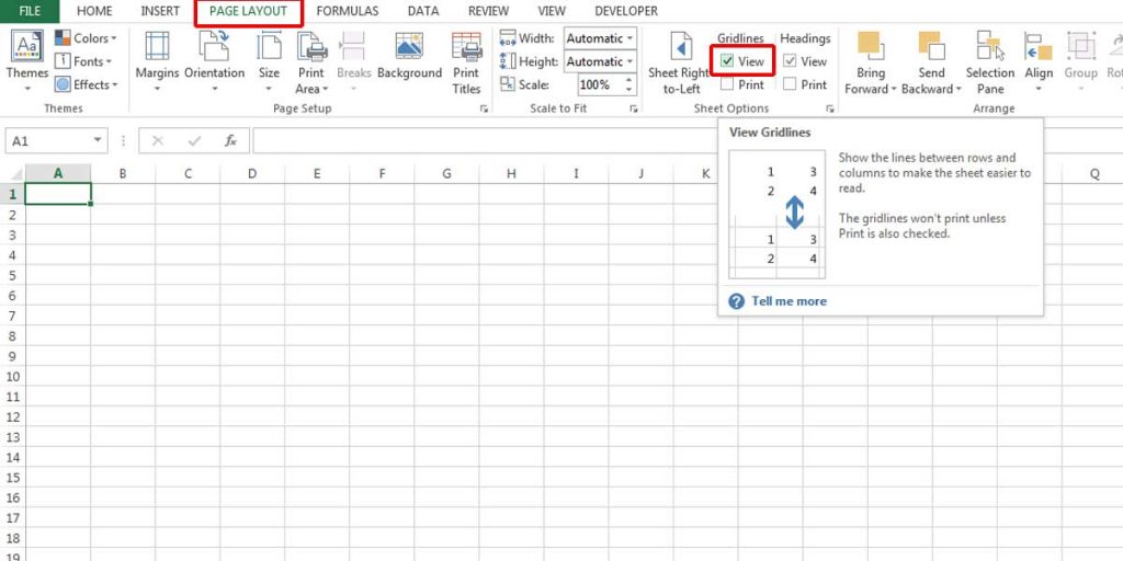
1. Go to the Page Layout tab.
2. Find Gridlines in the Sheet Options group. There are two options dedicated to gridlines and two for Headings, which are the numeric and alphabetic titles on the top and side of the worksheet.
3. To add gridlines in Excel, easily select View by clicking on its checkbox. The gridlines will be visible on the sheet.
4. If the headings have been hidden too, simply click on the View checkbox on the Headings group.

Method 2- Adding Gridlines In Excel Via The View Tab 

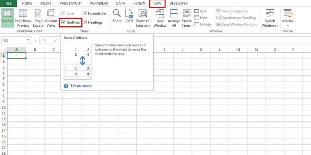
1. Go to the Show group in the View tab. 
2. Simply select the Gridlines checkbox.

How To Remove Gridlines In Excel?

Method 1- Removing Gridlines In Excel Via Page Layout

Hiding Excel gridlines is as easy as adding them. 

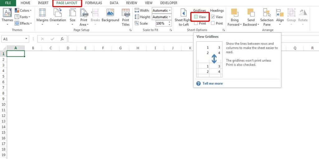
1. Go to the Sheet Options group in the Page Layout tab.
2. Uncheck the checkbox of View under the Gridlines title.
3. If you want to hide the headings too, you can deselect the View checkbox under the Heading title too.
4. Now you have a plain Excel sheet. Although the grids are not visible, the sheet still has its cells like before.

Method 2- Removing Excel Grids In The View Tab

Just go to the View tab and uncheck the Gridline checkbox in the Show group. 

Method 3- Change The Background Color 

This is another trick to hide the gridlines in Excel. 

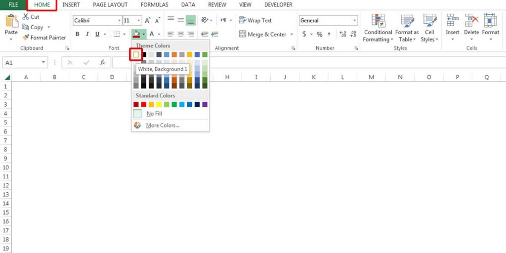
1. Select all the cells by pressing Ctrl + A keys.
2. Go to the Home tab and change the background color to white.

Method 4- Hiding The Gridlines In Excel Using The Shortcut Key

There is a shortcut to hide the gridlines in the Excel sheet. You only need to press the”Alt + W+V+G” keys on the sheet, and you can see the grids fade away.

You can press the keys again to show the grids on the Excel sheet. 

Why  Hide The Gridlines In Excel?

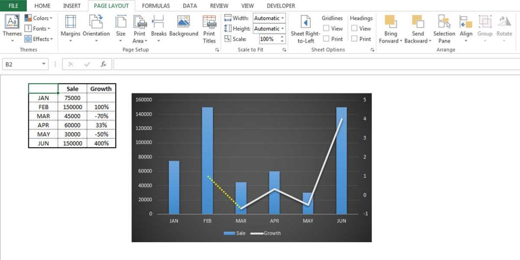
You may think about why we need to hide the grids in Excel? That’s simple; it makes your sheet more presentable. However, it will be easier to insert your data in the Excel sheet while it has its gridlines. Then, after finishing your report, you can make the grids invisible to make it more understandable and clear to read, especially when you have a chart on the page.

How To Print Excel With Gridlines? 

Normally, Excel sheets are printed without their grids unless you have made a table that fills all the cells. Needless to say, you can print gridlines in Excel too.

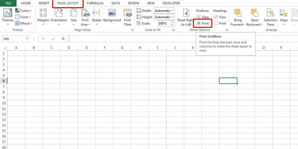
1. Go to the Page Layout tab. 
2. Select the Print checkbox under the Gridlines title. You can also print your worksheet with their headings by selecting the Print checkbox under the Headings Title.

There is also another way to print the gridlines in Excel. 

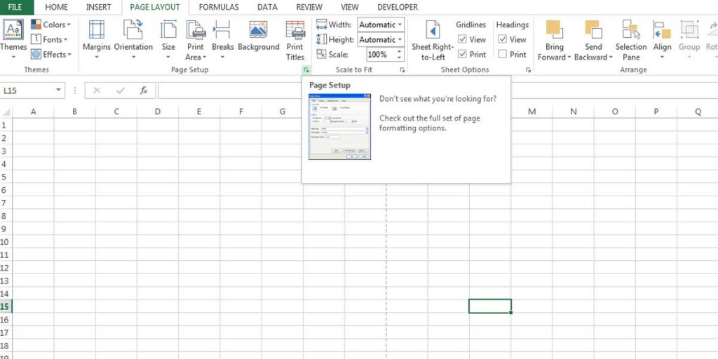
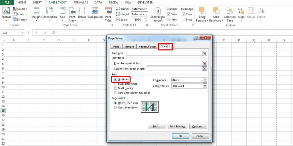
1. Go to the Page Setup group under the Page Layout tab. 
2. Click on the small arrow in the corner of the Page Setup block to open the settings.

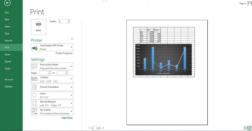
3. You can also access “Page Setup” from the Print action. To do so, go to File, click on Print, and select Page Setup on the bottom.

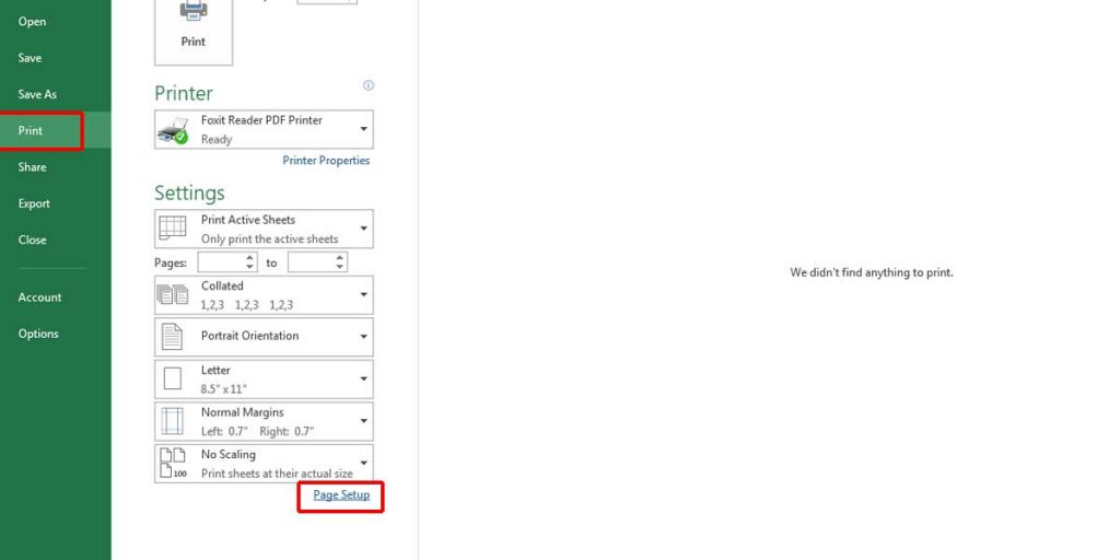
4. Go to the Sheet tab and select the Gridlines under the Print group. 

Bottom Line

Gridlines are the basic and known lines in the Excel sheet that can organize the data and guide you in your work. But sometimes, you may need to hide them to make your sheet clearer. In this post, we explained how to add, remove, and print gridlines in Excel using different methods.