How to Compare Two Columns in Excel: 4 Methods

Working in Excel is enjoyable and easy, especially if you know the tricks and techniques to work with different options. While having a table full of data, sometimes, you may need to make some comparisons. Whether it’s a comparison of a whole table or row by row, here are four methods of comparing two columns in Excel that can help you

1- Comparing two columns in Excel row by row 

TRUE/FALSE method 

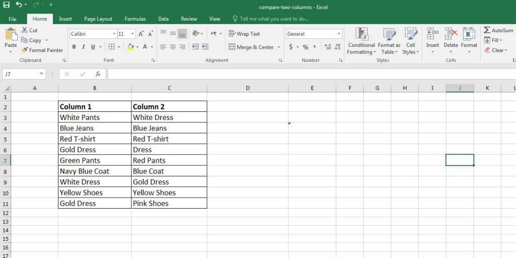
In this method, you can find out if the data in one row in a column is equal to the same row in the next column. For example, you may need to know if C3 is the same as B3. Check out the table below:

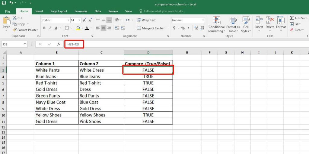
Let’s compare the data in columns B and C, row by row. First, select a column to see the results. We have chosen column D as the result column. This comparison is so easy. You only need to write a simple formula in the formula bar: (=B3=C3). This will check the data in both cells and give two results: TRUE and FALSE. Remember, you can drag the formula cell to the end of the table, so the formula is applied on all rows.

Using IF formula method to match two columns in excel

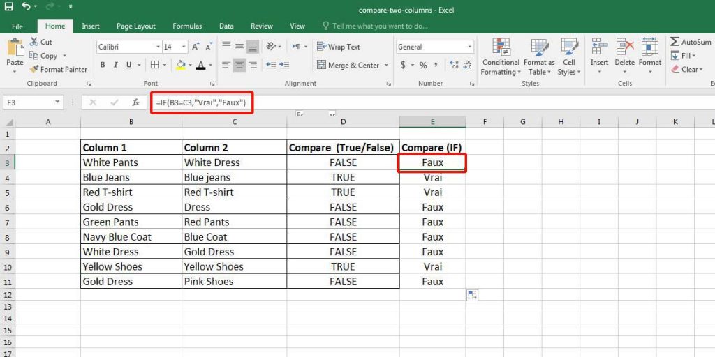
Sometimes, you may need to have an exact string after comparing two columns in Excel, or you may need to have a result with a particular text. For example, you may need to see ‘Match’ if the cells have the same data or ‘NO’ to say the data are not equal. Or even a word in a language other than English. Therefore, the first method is not for you because it has a predefined text result. In this case, you can write a simple IF formula.

=IF(B3=C3,”Vrai”,” Faux”)

Note: You can write whatever you want as a result instead of “Vrai” and “Faux.”

See the result below:

Please note that this formula doesn’t make a case-sensitive comparison. Thus, if any character in upper-case is important for your comparison, you can use this formula:

=IF(EXACT(B4,C4),”Vrai”,”Faux”)

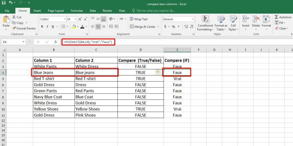
As you see, in this formula, “Blue Jeans” and “Blue jeans” are not the same.

Boost your productivity by getting a free consultation from Excel experts, and discover tailored solutions to optimize your data management and analysis

 

Highlighting Matched Data in One Row

Comparing two columns in Excel can also be done by highlighting the matched data. We can highlight them in the following steps: 

1. Select the table or the columns you want to compare. 
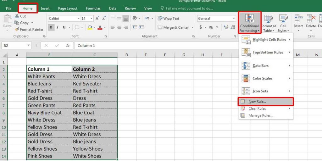
2. Click on the “Home” tab and click on the “Conditional Formatting” option, in the Styles group. Then, select “New Rule.”

   

3. You will see a dialogue box with different options. Select “Use a formula to determine which cells to format.”
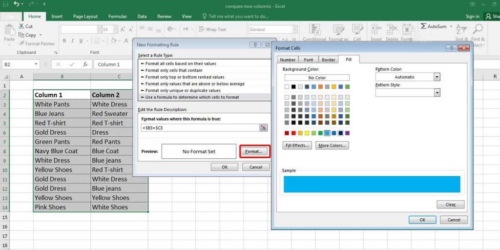
4. In the formula field, write the following formula: =$B3=$C3. Note that the formula may change based on the columns you have. In our example, we wanted to check these two columns (B and C) and our data starts from row 3. 
5. In the next step, you need to choose a format for highlighting. Therefore, click on the “Format” button. The Format Cells dialog box will open. Now you can change font color, border, or just choose a Fill color.

   

6. Click “OK” to see the result. 

2- Comparing two columns in Excel by Highlighting

Highlighting Matched Data in Different Rows 

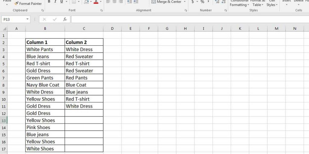
This method is different from what we did in the previous one. Sometimes the matched data might not be in the same rows of a table. Therefore, you need to compare two columns but not row by row. Check the table below.

In this case, you can find and highlight the matches following these steps: 

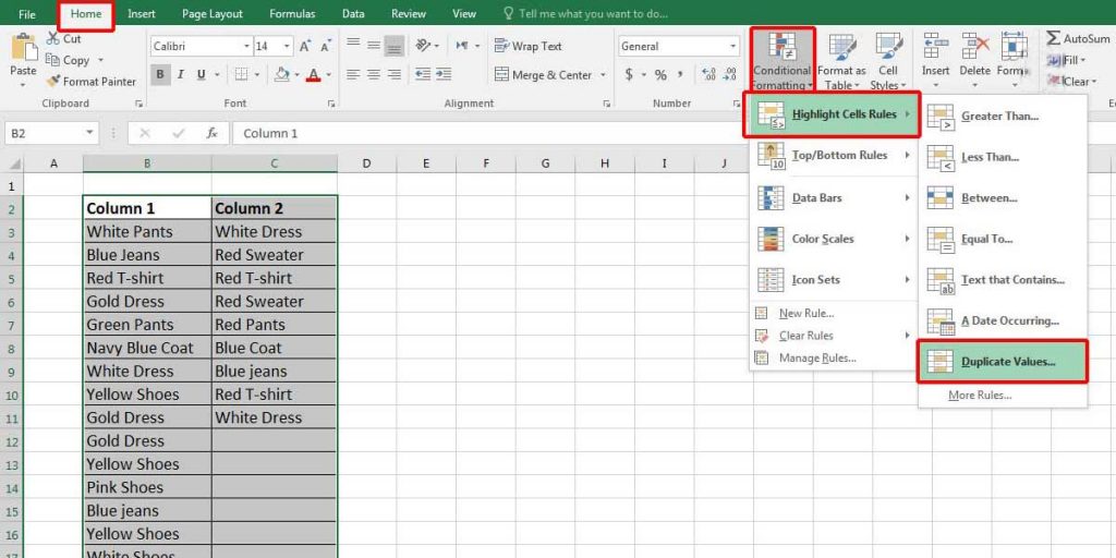
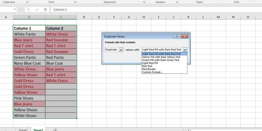
1. After selecting the dataset, go to the Home tab and click on the “Conditional Formatting”, in the Styles group. A drop-down list will open. This time, click on “Highlight Cells Rules” and select “Duplicate Values.”

   

2. A dialogue box will open with predefined values. You can select the highlighting format in the second drop-down.

   

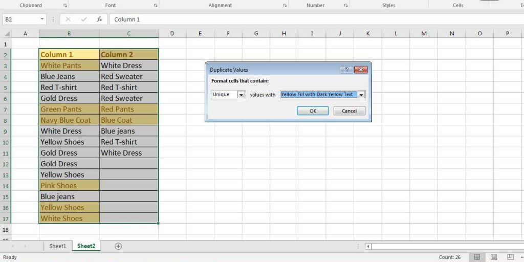
Highlighting Mismatched Data in Different Rows

This time we are going to compare two columns in Excel and highlight the data that are not matched. If you have done the previous steps correctly, it will be easy to find the unique data in the second step. See the following image.

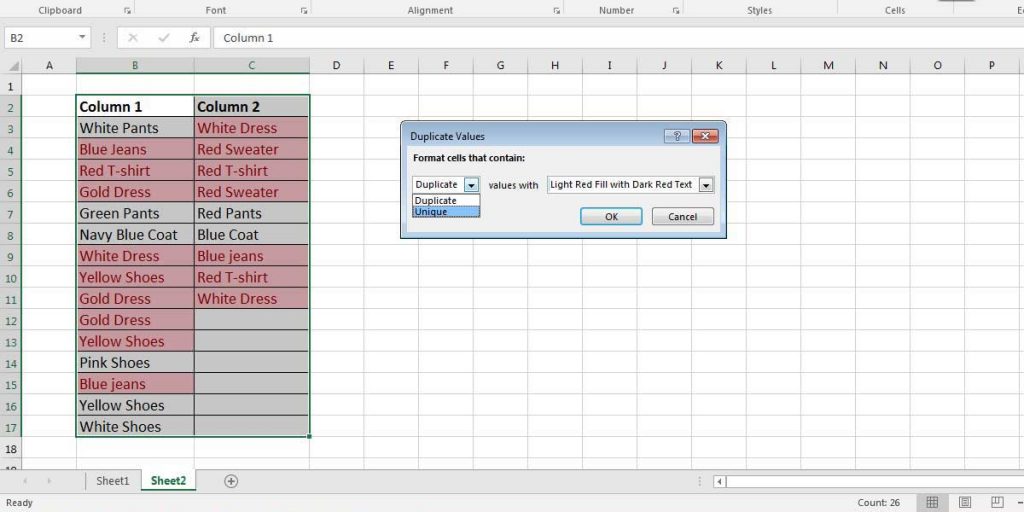
You only need to select “Unique” from the drop-down menu and choose the formatting for its highlight. You will see the following result:

3- Comparing Two Columns in Excel to Find Missing Data 

This time, we want to compare two columns and find data in the first column that are not available on any rows of the second column. Let’s see what column B has that column C doesn’t have.

Enhance your software capabilities with our customizable Add-In Solutions, seamlessly integrating new features to meet your business needs.

VLOOKUP Function | Using Vlookup to Match Data

One way to find the missing data in two columns is using the VLOOKUP function. The formula is as follow: 

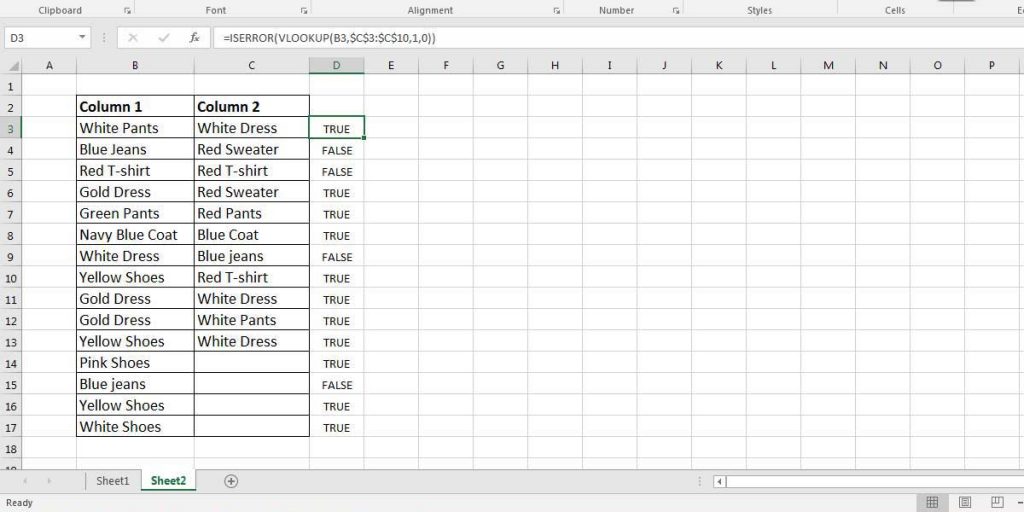
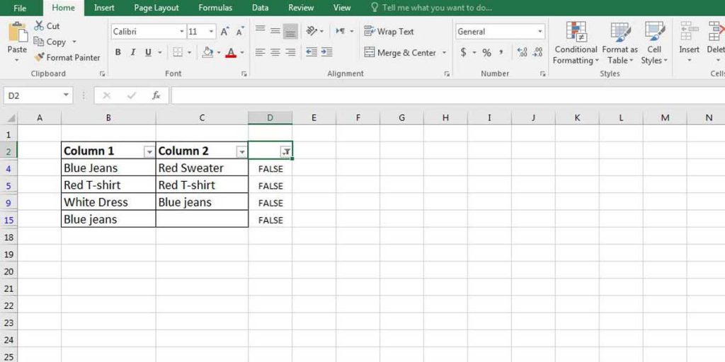
=ISERROR(VLOOKUP(B3,$C$3:$C$10,1,0))

In this formula, B3 is the base column that we want to compare with C3 to C10. The result of this formula is shown by TRUE or FALSE. If you see TRUE, it means the data on that row can be found on the second column too. FALSE shows that the data in column B can’t be found on any rows of column C. 

Therefore, in our example, we can find White Pants in Column C, but there is no “Blue Jeans” in that column. Moreover, this comparison method is case-sensitive, so it doesn’t count the “Blue jeans” that appear in column C.

If you have a lot of data on this table, you can filter the result column to see only the missing data. 

If you want to read more about using Vlookup to handle large excel files, you can read our article about Handle Large Excel Files With VLookup Formulas.

Match Function 

This method is quite similar to the VLOOKUP function. You will reach the same result in both these methods. The formula is as follow: 

=NOT(ISNUMBER(MATCH(B3,$C$2:$C$10,0)))

Related post: Combination Of INDEX And MATCH Functions In Excel

4- Comparing Two Columns and Pulling the Matching Data

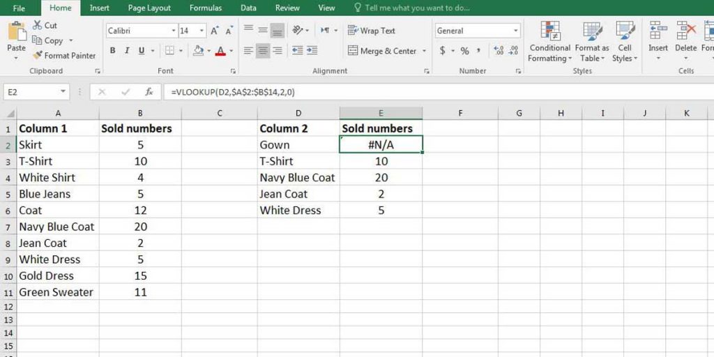
You may need to compare two columns in different tables and pull out the values. Suppose you have the following datasheet about a monthly sale. Now you want to see how many of the exact products you have sold that month. This formula can help you find out:

 =VLOOKUP(D2,$A$2:$B$14,2,0)

The result will be:

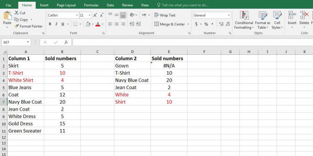
There is still one other condition that we may need to learn about. Since the previous formula only fetches the data of the cells with the exact match, we may need another formula that can specify the data of the cells that only are partially equal to each other. For example, “White” and “White shirts.” With this formula, even if we write “White,” Excel supposes we mean “White Shirt” (the first partially equal value).

The formula is: 

=VLOOKUP(“*”&D2&”*”,$A$2:$B$14,2,0)

The result is:

Bottom Line 

Comparing two columns in Excel is absolutely essential, especially when you have a huge table or set of data containing lots of values. These methods can help you find the needed values in a short time. Therefore, you can surely speed up your process by learning different tricks and techniques in Excel.