Mastering Advanced Excel Functions: Unleash Your Spreadsheet Superpowers

In today’s digital age, mastering Excel goes beyond the basics. Understanding and utilizing advanced Excel functions can transform your spreadsheet experience, making you a true Excel superhero. In this blog, we’ll explore the depths of Excel’s capabilities, delving into essential advanced functions, practical use cases, and expert tips. Join us to walk through Excel advanced features, functions, and formulas.

Explanation of Advanced Excel Functions

Firstly, let’s clarify what Excel functions are. In Excel, functions are predefined formulas that perform calculations using specific values in a particular order. They can range from basic arithmetic operations such as summing up the numbers to complex logical analyses specified in finance, statistics, or other fields. advanced Excel functions, as the name suggests, go beyond the fundamental operations, allowing users to perform intricate tasks with ease.

These Excel functions are broadly categorized into different groups:

• Text functions
• Math functions
• Logical functions
• Date and time functions
• Lookup and reference functions
• Array functions

Each item of the Excel functions list serves a unique purpose, empowering users to manipulate and analyze data efficiently.

Common Use Cases

Imagine you’re working with vast datasets and need to find specific information quickly. Advanced Excel functions can come to your rescue. Let’s say you’re managing a sales database and want to calculate the total revenue generated by a specific product category within a certain timeframe. Advanced functions like SUMIFS can solve this complex problem effortlessly, saving you valuable time and energy.

In the field of human resources, advanced Excel functions play a vital role in managing employee data. Imagine you have a large dataset containing employee information, including hire dates, departments, and salaries. With VLOOKUP, you can streamline the process of cross-referencing this data. For instance, when conducting performance reviews, you can use VLOOKUP to quickly find an employee’s department and tenure.

In educational institutions, particularly for educators and administrators dealing with student data, Excel functions are incredibly beneficial. For example, calculating the average scores of students in various subjects using AVERAGEIF based on specific criteria such as grade level or subject type enables educators to identify areas where students may need additional support. Similarly, administrative staff can utilize functions like INDEX and MATCH to streamline enrollment processes, ensuring students are placed in appropriate classes based on their academic records.

Let’s delve deeper into each function group!

Text Functions

These advanced Excel functions including CONCATENATE, SUBSTITUTE, and TEXT, are invaluable for manipulating textual data. For instance, suppose you have a list of names in different formats and want to standardize them. The CONCATENATE function can help merge first and last names seamlessly, ensuring consistency in your database.

– CONCATENATE

• Combines two or more text strings into one.

Syntax: =CONCATENATE(text1, text2,…)

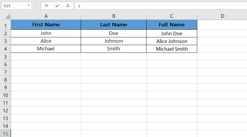
Let’s see how to concatenate in Excel. Suppose that you have a list of customers’ first names and last names in separate columns, and you want to combine them in one single cell. You can use the CONCATENATE function to do so:

=CONCATENATE(“John”, ” “, “Doe”) results in “John Doe”.

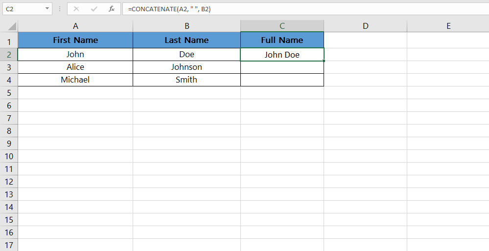
After entering the formula in cell C2, press Enter. Excel will concatenate the first name from cell A2, add a space, and then concatenate the last name from cell B2. Drag the fill handle (a small square at the bottom-right corner of the cell) down to apply the formula to other cells in column C.

– SUBSTITUTE

• Replaces specific text in a text string with new text.

Syntax: =SUBSTITUTE(Cell Address, old_text, New_text)

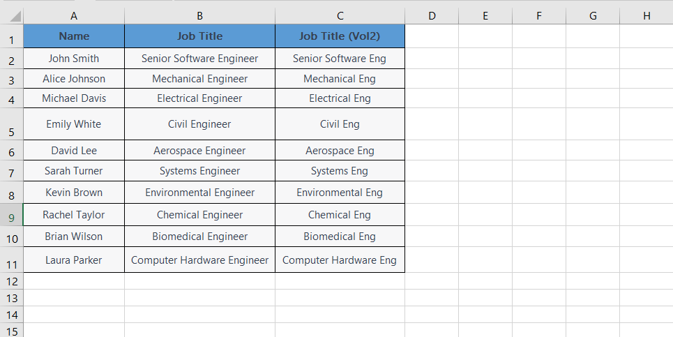
Imagine you have a list of employees with their job titles.

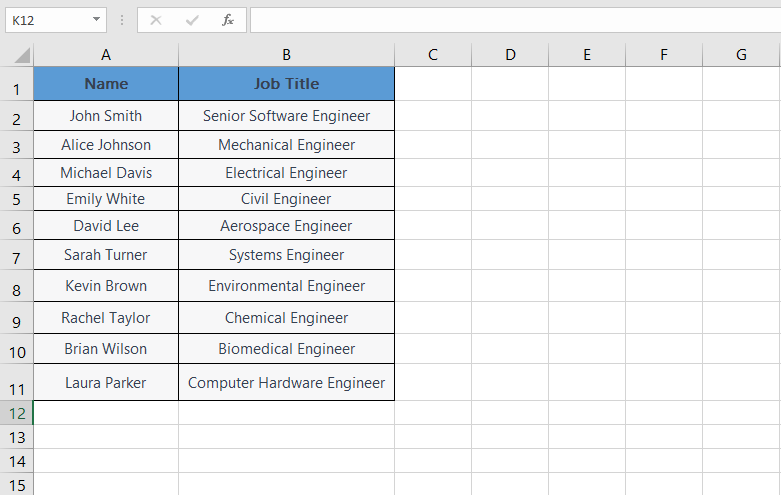
If you want to substitute “Engineer” with its abbreviated version (Eng), you can use this function:

=SUBSTITUTE(B2, “Engineer”, “Eng”)

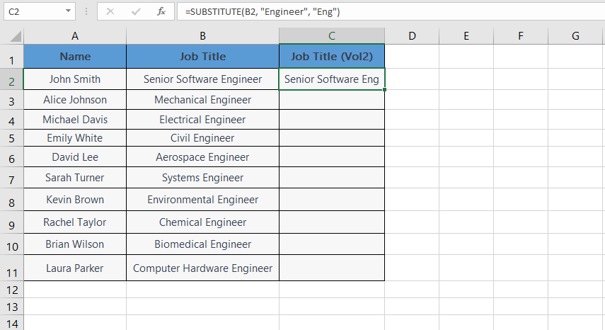
Drag the fill handle down to apply the formula to other cells in column C.

Now we have another data table:

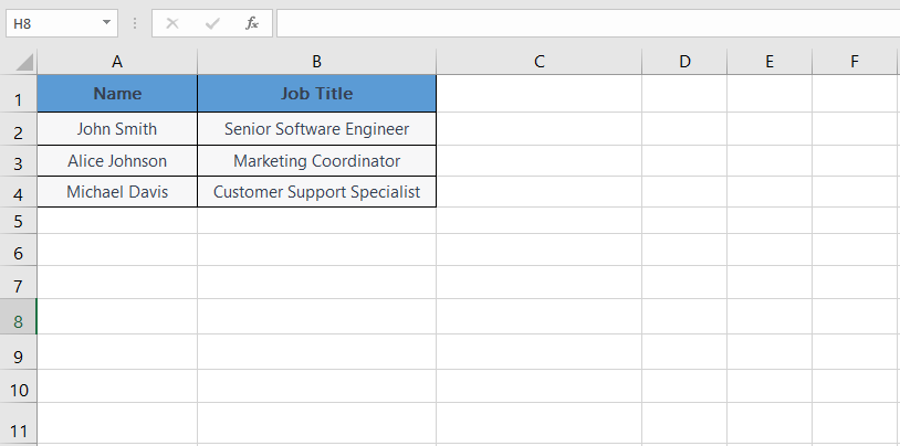
Let’s say you want to abbreviate the words “Senior” as “Sr.”, “Engineer” as “Eng.”, “Marketing” as “Mktg”, and “Specialist” as “Spec.” within the same cell.

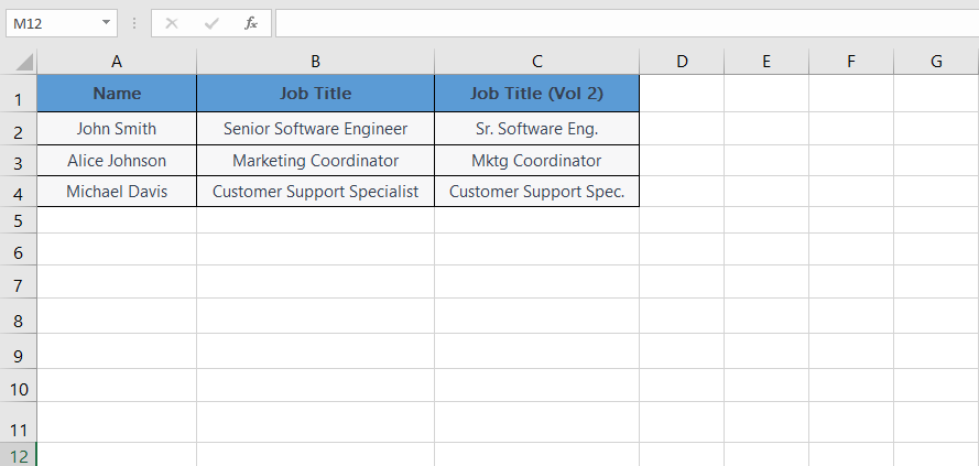
In cell C2, you can use the SUBSTITUTE function to replace the specified words with their abbreviations:

=SUBSTITUTE(SUBSTITUTE(SUBSTITUTE(SUBSTITUTE(A2, “Senior”, “Sr.”), “Engineer”, “Eng.”), “Marketing”, “Mktg”), “Specialist”, “Spec.”)

Drag the fill handle down to apply the formula to other cells in column C.

– TEXT

• Converts a value to text with a specified number format. It allows you to customize the way dates, numbers, and text are displayed in Excel, providing you with flexibility in presenting your data.

Syntax: =TEXT(value, format_text)

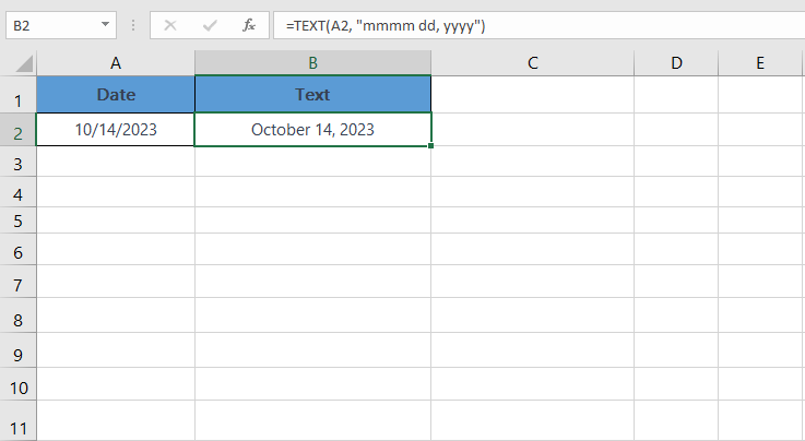
Let’s say you have a date in cell A2: 10/14/2023. If you want to format this date as “October 14, 2023” you just need to choose “TEXT” from the list of advanced Excel functions and use this formula:

=TEXT(A2, “mmmm dd, yyyy”)

After entering the formula in cell B2, Excel will format the date and display it as October 14, 2023.

Math and Statistical Functions

Advanced Excel functions related to math and statistics like SUMIFS, AVERAGEIFS, and RANK empower you to perform in-depth data analysis. For example, you might want to calculate the average sales figures for a specific product category during the last quarter. AVERAGEIFS allows you to specify multiple criteria, providing precise results for your analysis.

– SUMIFS

• Adds the cells specified by multiple conditions.

Syntax: =SUMIFS(sum_range, criteria_range1, criteria1, [criteria_range2, criteria2], …)

Let’s say you have a list of sales data for different products.

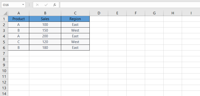
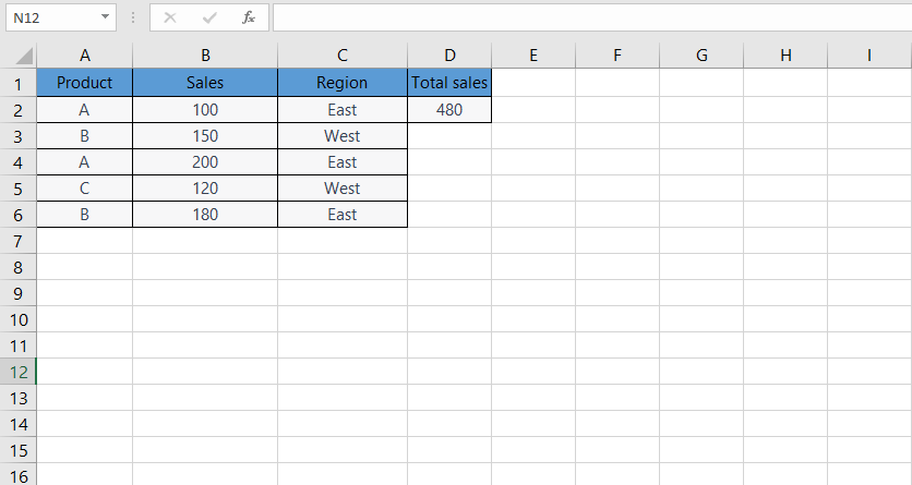
Now, you want to calculate the total sales for products in the “East” region. You can use the SUMIF function to achieve this.

=SUMIF(C2:C6, “East”, B2:B6)

In this formula:

• C2:C6 represents the range containing the regions.
• “East” is the criteria you are using to sum the sales.
• B2:B6 represents the range containing the sales amounts.

After entering the formula, Excel will calculate the total sales for products in the “East” region.

– AVERAGEIFS

• Calculates the average of cells specified by multiple conditions.

Syntax: =AVERAGEIFS(average_range, criteria_range1, criteria1, [criteria_range2, criteria2], …)

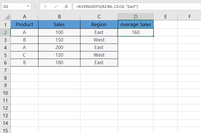
In the previous data table, let’s calculate average in Excel for products’ sales in the “East” region. You can use this function to find the average sales based on the criteria “East” in column C:

=AVERAGEIFS(B2:B6, C2:C6, “East”)

– RANK

• Returns the rank of a number in a list of numbers.

Syntax: =RANK(number, ref, [order])

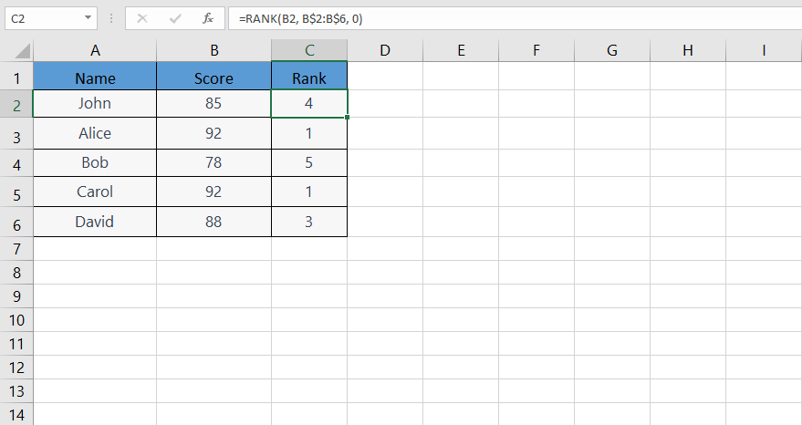
Imagine you have a list of student names with their corresponding exam scores.

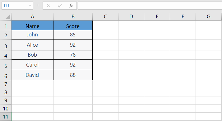
You want to calculate the rank of each student’s score in column B, using advanced Excel functions. To do this, you can use the RANK function. To rank the scores in descending order, enter the following formula in cell C2, and drag it down to apply to other cells in column C:

=RANK(B2, B$2:B$6, 0)

Date and Time Functions

Excel’s date and time functions, such as DATE, TIME, and EOMONTH, facilitate efficient handling of temporal data.

– DATE 

• Returns the serial number of a particular date.

Syntax: =DATE(year, month, day)

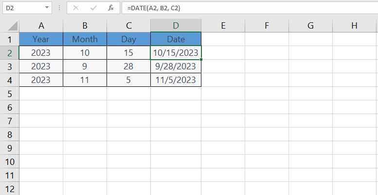
You have a list of task completion dates in three separate columns, and you want to combine these columns into a single date column:

=DATE(A2, B2, C2)

– TIME

• Returns the serial number of a particular time.

Syntax: =TIME(hour, minute, second)

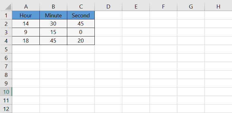
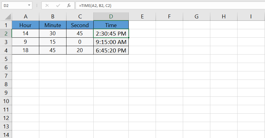
In the fourth column, we will use the TIME function to display the time based on the values in the first three columns.

=TIME(A2, B2, C2)

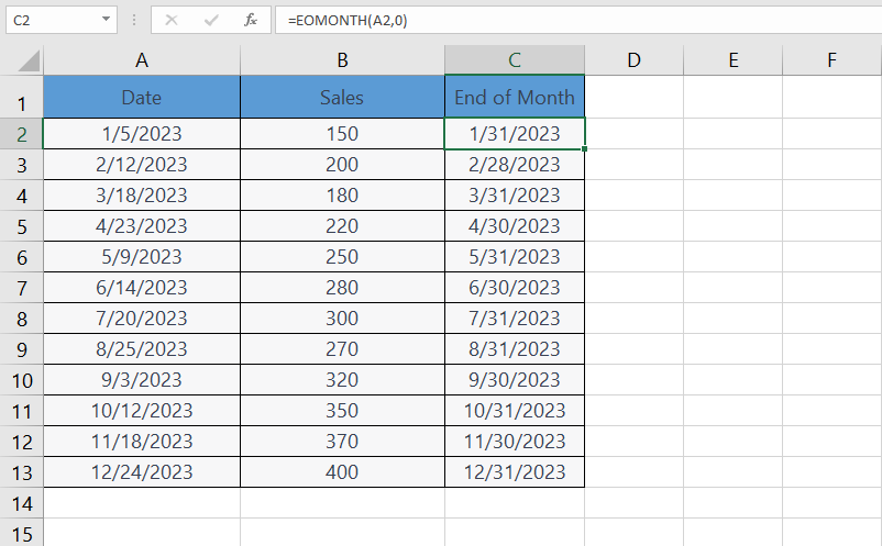
– EOMONTH

• Returns the serial number of the last day of the month before or after a specified number of months.

Syntax: =EOMONTH(start_date, months)

• start_date: This is the initial date from which you want to calculate the end of the month.
• months: This is the number of months before or after the start date. Use positive values for future months and negative values for past months.

Suppose you have a list of sales data for a year, and you want to calculate the end of the month for each month in the sales data. Your data might look like this:

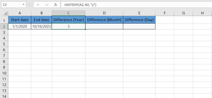
– DATEDIF

• Calculates the difference between two dates in years, months, or days.

Syntax: =DATEDIF(start_date, end_date, unit)

• start_date: The start date in Excel date format.
• end_date: The end date in Excel date format.
• unit: A three-letter code specifying the time unit (“y” for years, “m” for months, and “d” for days).

Let’s say you have a start date in cell A2 (01/01/2020) and an end date in cell B2 (10/16/2023). You want to use advanced Excel functions for calculating the difference in years, months, and days between these two dates.

To calculate the difference in years:

=DATEDIF(A2, B2, “y”)

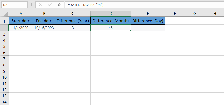
To calculate the difference in months:

=DATEDIF(A2, B2, “m”)

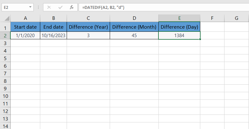
To calculate the difference in days:

=DATEDIF(A2, B2, “d”)

In the mentioned case, the difference in years, months, and days are independent from each other. If you want the difference between two dates to be expressed in the format of “X years, Y months, and Z days” you can use this formula:

=DATEDIF(A2, B2, “y”) & ” years, ” & DATEDIF(A2, B2, “ym”) & ” months, and ” & DATEDIF(A2, B2, “md”) & ” days”

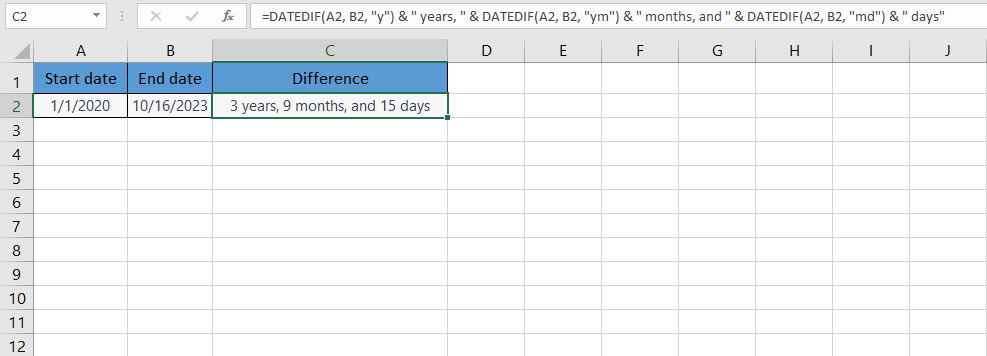
This formula uses the DATEDIF function to calculate the difference in years, months, and days between the two dates.  

Lookup and Reference Functions

In a scenario where you have data distributed across multiple sheets or workbooks, advanced lookup and reference functions like VLOOKUP, HLOOKUP, INDEX, and MATCH are indispensable. These functions enable you to cross-reference data seamlessly, ensuring accurate analysis and reporting.

– VLOOKUP

• Searches for a value in the first column of a table and returns a value in the same row from another column.

Syntax: =VLOOKUP(lookup_value, table_array, col_index_num, [range_lookup])

Let’s say you have a list of products and their corresponding prices in a table.

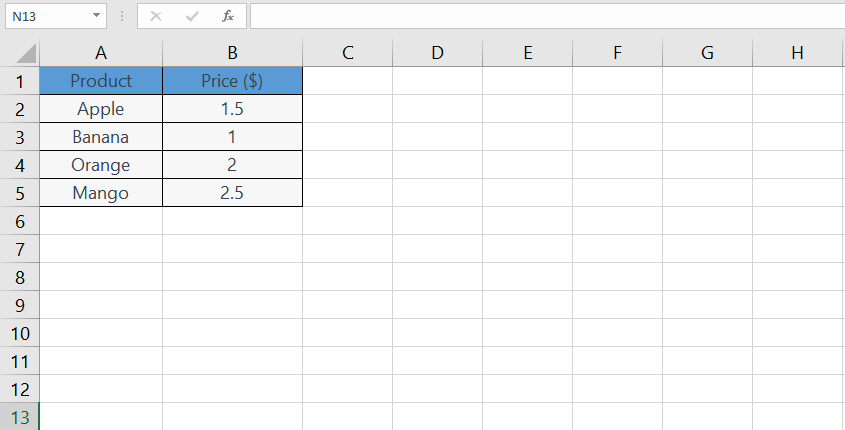
There is a separate list of orders with product names and you want to fetch the prices from the above table for each product.

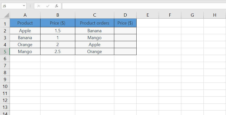
In cell D2 (next to “Banana”), you can use the VLOOKUP function to find the price for “Banana” from the products table:

=VLOOKUP(C2, $A$2:$B$5, 2, FALSE)

In this formula:

• “C2” is the lookup value (the product name “Banana” in this case).
• “$A$2:$B$5” represents the table range where Excel will search for the product name and corresponding price.
• “2” specifies that the function should return the value from the second column of the table (the price column).
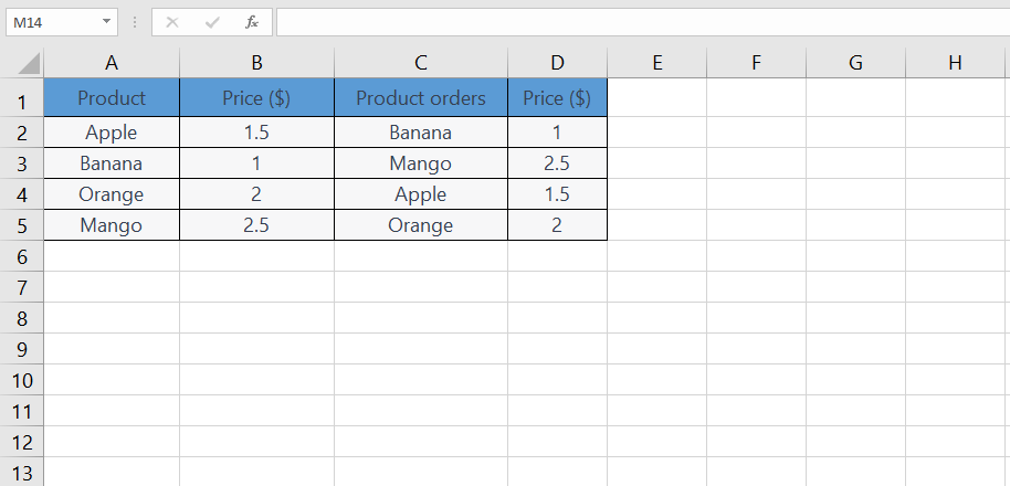
• “FALSE” indicates an exact match.

Drag the formula down from E2 to E5 to fill the prices for all products.

– HLOOKUP 

• Searches for a value in the first row of a table and returns a value in the same column from another row.

Syntax: =HLOOKUP(lookup_value, table_array, row_index_num, [range_lookup])

We have this data table with product names and order numbers:

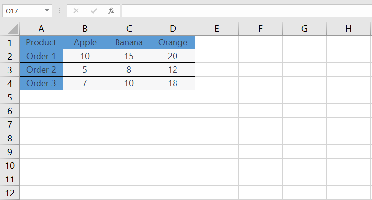
To find the quantity of Bananas ordered in “Order 1” with advanced Excel functions, we can use the HLOOKUP function:

=HLOOKUP(“Banana”, A1:D4, 2, FALSE)

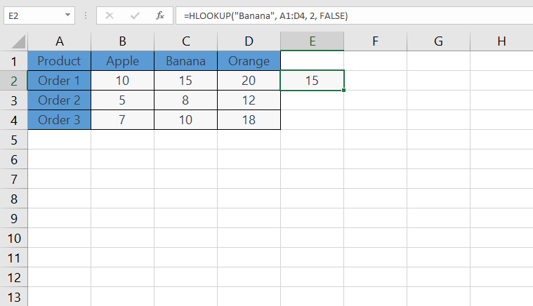
In this formula:

• “Banana” is the lookup value (the product name you want to find).
• “A1:D4” represents the table range where Excel will search for the product name.
• “2” specifies that the function should return the value from the second row of the table (the quantity column for Bananas).
• “FALSE” indicates an exact match.

– INDEX

• Returns the value of a cell in a specific row and column of a range.

Syntax: =INDEX(array, row_num, [column_num])

Consider a similar table with product names, corresponding prices, and quantities sold:

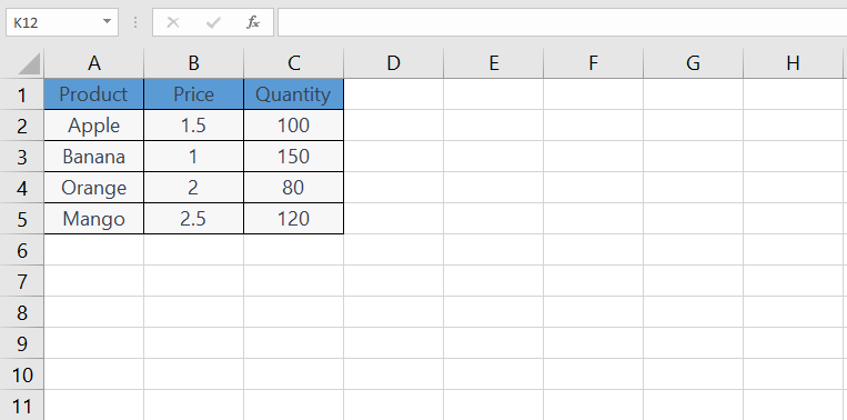
You can use the INDEX function to find the price of “Banana” in cell D2:

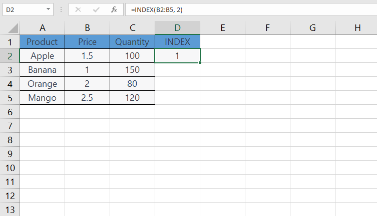
In this formula:

• “B2:B5” represents the range of prices.
• “2” represents the row number where “Banana” is located in column A.
• The “INDEX” function retrieves the price from the second row of the specified range.

Now, let’s say you want to find the quantity sold for “Orange”. You can use the INDEX function in cell D3:

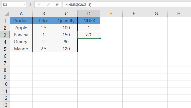
In this formula, “C2:C5” represents the range of quantities sold, and “3” represents the row number where “Orange” is located in column A.

– MATCH

• Searches for a specified value in a range and returns the relative position of that item.

Syntax: =MATCH(lookup_value, lookup_array, [match_type])

Let’s consider a list of cities and their corresponding populations.

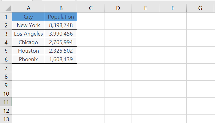
To find the position of the city “Chicago” in the list, you can use the MATCH function in cell C2:

=MATCH(“Chicago”, A2:A6, 0)

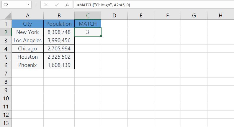
• “Chicago” is the lookup value.
• “A2:A6” represents the range where Excel will search for the city name.
• “0” indicates an exact match.

 

 

Logical Functions

Among Excel spreadsheet functions, Logical functions, including IF, AND, OR, and NOT, allow you to create sophisticated decision-making processes within Excel.

– IF 

• Performs a logical test and returns one value if the condition is true and another if false.

Syntax: =IF(logical_test, value_if_true, value_if_false)

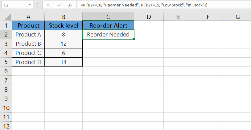
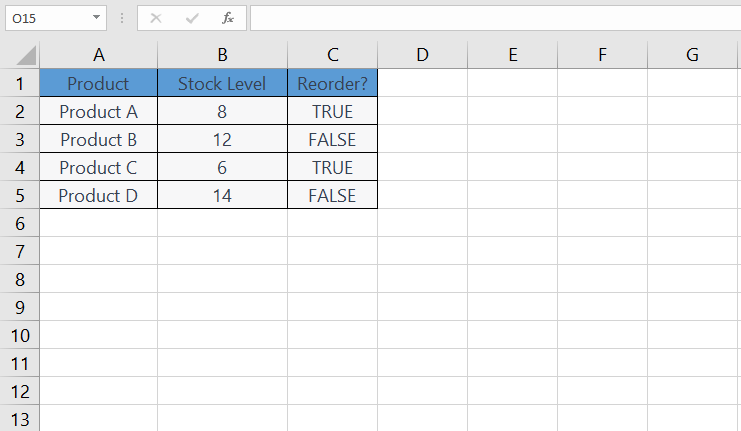
Suppose you’re managing inventory and want to automate reorder decisions, relying on advanced Excel functions. By using nested IF statements, you can create a logical formula that triggers reorder alerts when stock levels fall below a specified threshold.

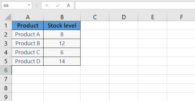
In column C, you can create a formula using nested IF statements to generate reorder alerts when stock levels fall below the threshold of 10 units. The formula checks each product’s stock level and provides a message based on the condition.

=IF(B2<=10, “Reorder Needed”, IF(B2<=15, “Low Stock”, “In Stock”))

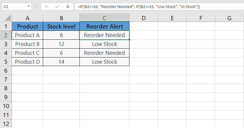
Here’s how the formula works:

• First IF Statement: Checks if the stock level (B2) is less than or equal to 10. If true, it returns “Reorder Needed”.
• Nested IF Statement: If the first condition is false, it checks if the stock level is less than or equal to 15. If true, it returns “Low Stock”.
• Default Case: If both conditions are false, it returns “In Stock”.

– AND

• Returns TRUE if all the conditions are true, and returns FALSE if any of the conditions are false.

Syntax: =AND(condition1, condition2, …)

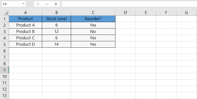
Let’s consider a list of products, their current stock levels, and their reorder status. You want to check if a product needs to be reordered based on the criteria that the stock level is less than 10, and the reorder status is “Yes”.

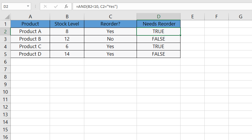
In cell D2, you can use the AND function to check if a product needs to be reordered based on the stock level and reorder status. Enter the following formula:

=AND(B2<10, C2=”Yes”)

This formula checks two conditions:

• B2<10 checks if the stock level is less than 10.
• C2=”Yes” checks if the reorder status is “Yes”.

The AND function returns TRUE only if both conditions are true.

After entering the formula in cell D2 and dragging it down, Excel will evaluate the conditions for each row:

– OR

• Returns TRUE if any of the conditions are true, and returns FALSE if all of the conditions are false. Excel OR Function performs in the same way as the AND function does.

Syntax: =OR(condition1, condition2, …)

– NOT

• Reverses the logical value of its argument. It returns TRUE if the expression is FALSE, and FALSE if the expression is TRUE.

Syntax: =NOT(logical)

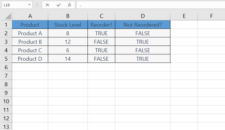
Let’s consider a list of products, their current stock levels, and a flag indicating if they need to be reordered. The “Reorder?” column contains TRUE for products that need to be reordered (stock level less than 10) and FALSE for products that do not.

In cell D2, you can use the NOT function to reverse the logical value in the “Reorder?” column:

=NOT(C2)

Array Functions

The last group of advanced Excel functions are Array functions. Functions like SUMPRODUCT and TRANSPOSE are powerful tools for working with arrays of data.

– SUMPRODUCT

• Multiplies corresponding components in the given arrays and returns the sum of those products.

Syntax: =SUMPRODUCT(array1, array2, …)

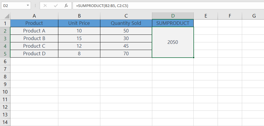
Let’s assume you have a list of products, their unit prices, and the quantities sold:

 

To calculate the total revenue generated from these sales, you can use the SUMPRODUCT function. The total revenue is calculated by multiplying the unit price of each product by the quantity sold and then summing up these values.

In cell D2, you can enter the following formula:

=SUMPRODUCT(B2:B5, C2:C5)

In this formula:

• B2:B5 represents the range of unit prices.
• C2:C5 represents the range of quantities sold.

– TRANSPOSE

• The TRANSPOSE function in Excel is used to change the orientation of a range of cells or an array. It switches the rows and columns of a given range, effectively transposing the data.

Syntax: =TRANSPOSE(array)

Let’s assume you have a table with products and their corresponding sales data for three months:

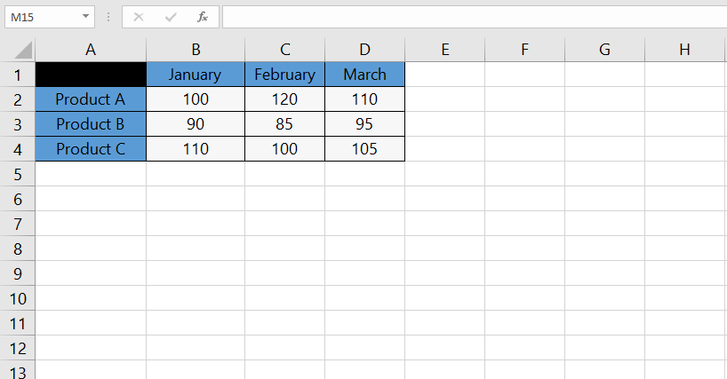
• Select the range where you want to paste the transposed data. For this example, you might select a new location in your worksheet.
• Enter the following formula in the first cell of the selected area, and press Ctrl+Shift+Enter to create an array formula:

=TRANSPOSE(A1:D4)

After entering the formula as an array formula, Excel will automatically transpose the data. The result will look like this:

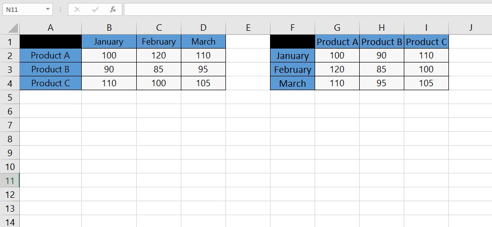
In this transposed table, the rows and columns have been switched with the help of advanced Excel functions.

 

 

Advanced Excel Functions Best Practices

To harness the full potential of Advanced Excel Functions explained before, consider these Excel formula tips:

• Efficient Formulas: Keep your formulas concise and efficient to enhance spreadsheet performance.
• Cell Referencing: Understand the differences between relative, absolute, and mixed cell references to avoid errors in your calculations.
• Error Handling: Implement error handling techniques like IFERROR to make your spreadsheets more robust.
• Documentation: Document your complex formulas for future reference, making it easier for others to understand your work.
• Regular Practice: Practice using advanced Excel functions regularly to build confidence and expertise.

Conclusion

In this blog, we’ve explored the vast world of Advanced Excel Functions step-by-step. By mastering these functions, you can streamline your workflow, perform complex calculations effortlessly, and make data-driven decisions with confidence. We encourage you to dive into the realm of advanced functions, experiment with different scenarios, and unlock the full potential of your Excel skills. If you have any questions, comments, or want to explore more about Excel Formula Tips, Excel Function Examples, or Excel Advanced Features, feel free to reach out.