Format Cells Option in Excel

What is the Format Cells Option in Excel?

By default, Excel has predefined formatting. When you enter data in each cell, the font, size, colour, and tabling are always the same unless you change them. Thus, you might need to make new formatting based on your preferences. That’s when the Format Cells option in Excel comes to the rescue!

Where to find Format Cells in Excel?

Using Format Cells options helps you change the appearance of the cells easily or even change a table in your Excel sheet to whatever pleases you. You only need to select and right-click on the cell (cells or table) you want to change.

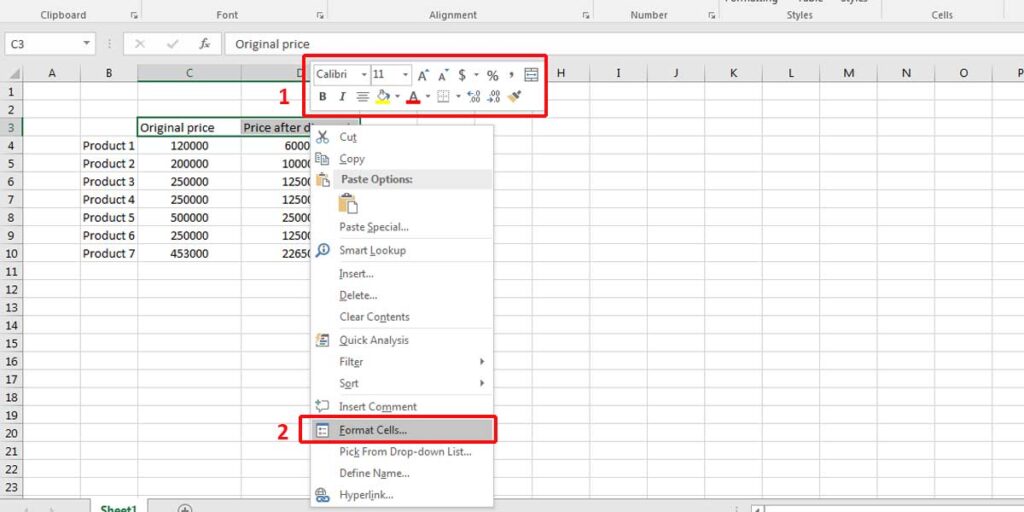
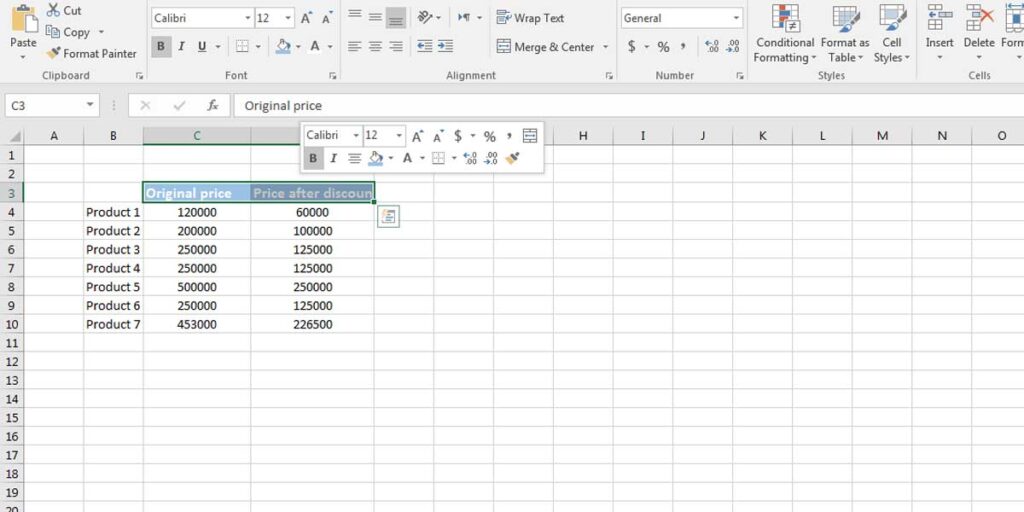
You can easily find some options to change the appearance of the selected cells on top of the list, such as cell colour, font theme, size, and colour. 

By clicking on the “Format Cells,” you can access more options, which are explained as follows. 

What are the six options in Format Cells?

After clicking on the “Format Cells,” a pane opens with six tabs: 

Tab 1- Number

This option is only applied to the cells with numerical values. Select the cells and choose the format that is listed under Category. By default, all the cells have a General format, no matter their value type. However, you can’t write formulas for the cells that are text or general. As a result, if you want to perform calculations on your form, it’s better to change the cell type to Number.

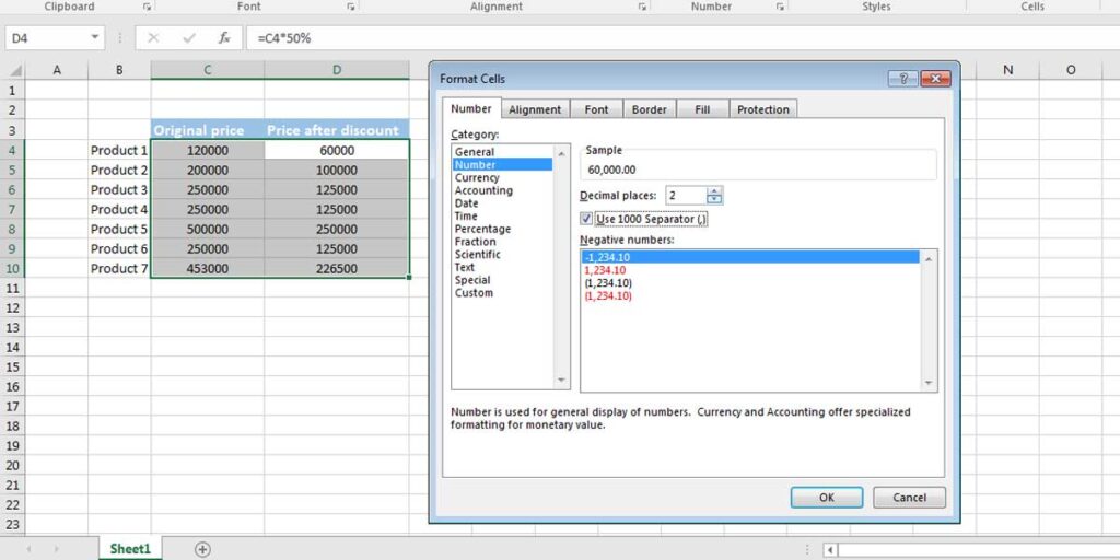
Each category type has different options that the users can choose based on their preferences. For example, they can add a separator, change the Decimal of a number or change currency type in the Currency section.

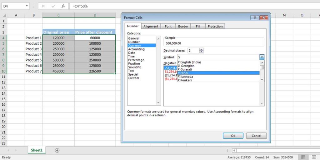
Before applying them to the cells, you can preview your changes under the Sample section.

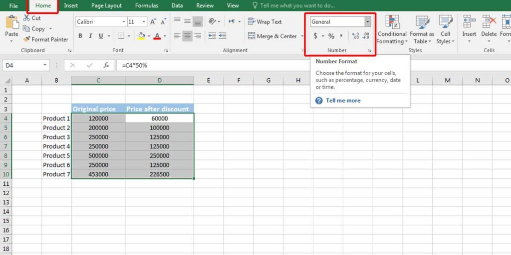
You can also have quick access to the most common options of the Number tab in the Number section of the Home tab. You only need to select the cells and choose Number Format. 

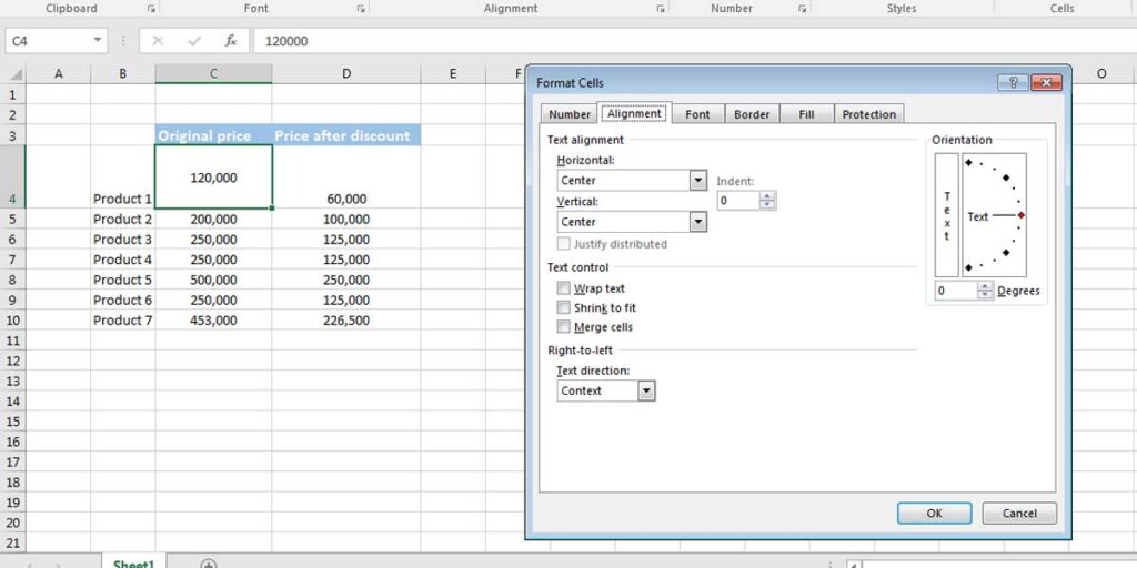
Tab 2 – Alignment

Excel has a default alignment for texts and numbers. Generally, texts are placed on the left side of the cell, and numbers are on the right. But you can change this on the Alignment tab on Format Cells. Any value on the cells can be aligned to the left, center, and right horizontally and top, center, bottom, justified, and distributed vertically.

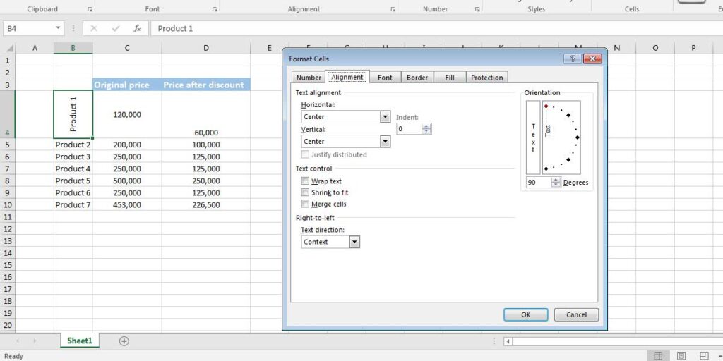
Moreover, you can even change the orientation of a value. Normally they are written horizontally, but you can change that to any degree you want. In our example, we changed it to 90 degrees. You can see the result below.

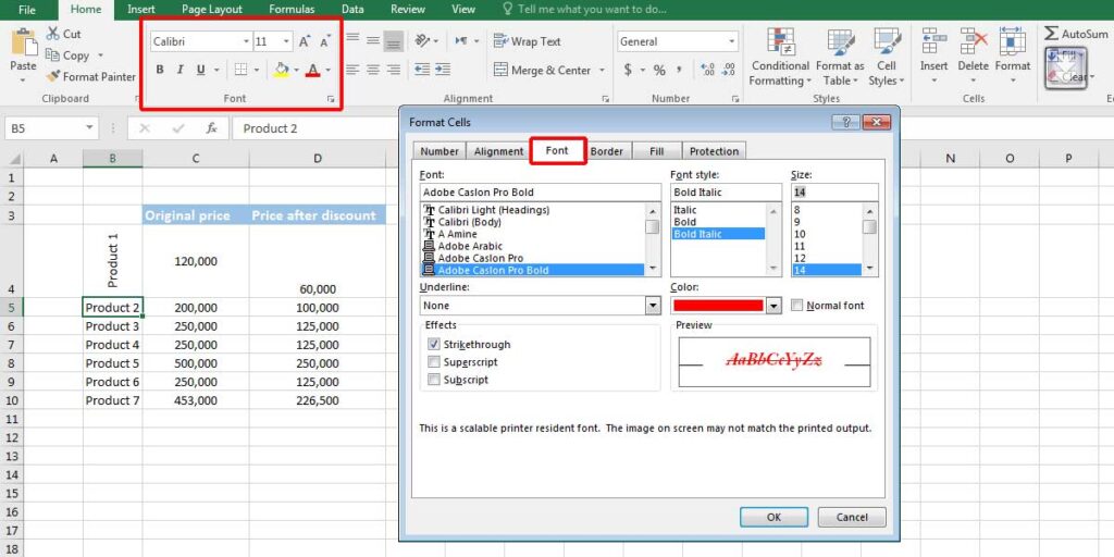
Tab 3 – Font

Changing the Font type or size is one of the most common functions in Excel, and it’s also quick and easy.

1. Select the cells you want to change their font options. 
2. Right-click and go to Format Cells. 
3. On the “Font” tab, there are all the options related to the fonts, like font type, font size, font style, font colour, and any effect you want to apply to the fonts. It is also possible to see a preview of any changes you make under the Preview section. 
4. Click Ok to apply the changes. 

Some of the most common options related to the fonts are quickly accessible in the Home tab under the Font section.

Tab 4 – Border 

Borders can help you improve the readability of your form. You can create a table or a form by creating borders around your data. Just select the area and go to the Format Cells option as you did in the previous steps. This time, select the Border tab.

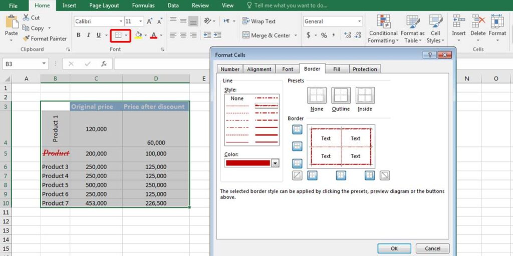
Borders also have different styles and sizes. Select the line style and create a suitable border. Click OK to apply the changes. 

Remember, it’s also possible to quickly create borders from the Home tab under the Font group. 

Tab 5 – Fill/Pattern 

Here is the fun part of the Format Cells in Excel because you can change the appearance of the cells by selecting a background colour or even a pattern. Select the cells and go to the Format Cells. Click on the Fill tab. In some versions of Excel, you may have this part under the Pattern section. The options are the same. 

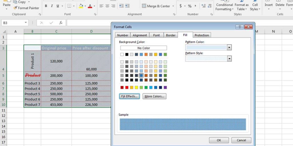
If you want your form to have a unique look, choose a pattern, or change the cell colour. The Sample section shows a preview of the selected cells.

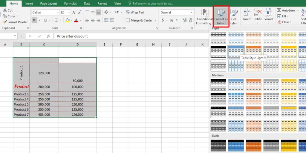
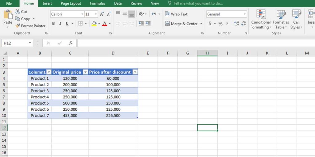
 Predefined Cell and Table Formats 

Although creating a table and changing the cell colour is completely customizable, it is possible to use predefined formatting. To use the default options, you don’t need to go to the Format Cells section; just select the area you want to define a format for, whether it’s one cell or a group of cells, which make a table. 

After selecting the cells:

If you want to create a table, go to the Styles group under the Home tab and click on Format as Table. A group of predefined table formatting opens. You can choose the one you prefer and change the appearance of the selected cells. 

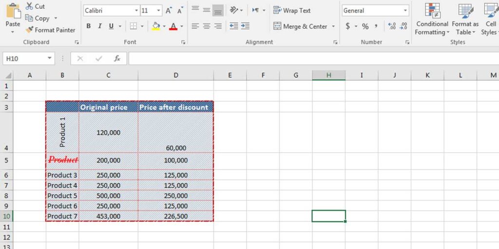
The result will be:

If you want to change only one cell’s appearance or would like to create your own-designed table, you can go to Cell Styles, located in the Styles group under the Home tab. A list of predefined formatting opens from where you can select your preferred cell style.

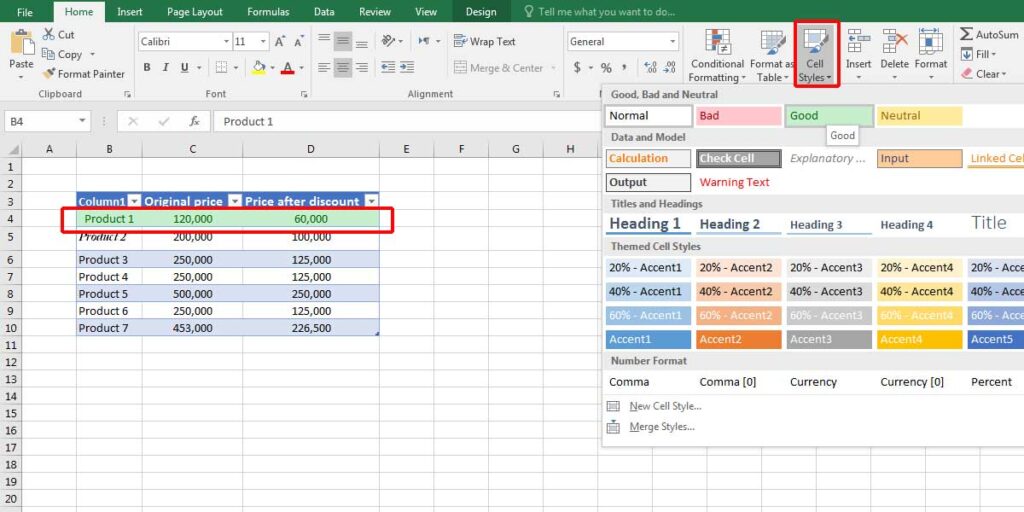
Format as Table option will give a header to the first row of the selected cell, which font colour and cell colour are different from the other cells. That’s the main difference between the Format as Table and Cell Styles. You can see the preview on the selected cells. 

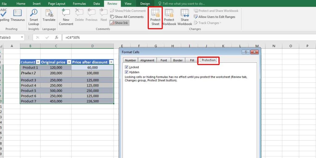
Tab 6 – Protection 

The last tab on the Format Cells group is the Protection tab, which only has two options: Locked and Hidden. If you want to lock your Excel sheet, you can select this checkbox. The hidden option will hide any formulas on this worksheet. 

However, this tab only works if you have already protected your worksheet. Therefore, select the options, go to the Review tab, and click on Protect Sheet. If any other user opens this file, they won’t be able to make any changes to this sheet.

Click on the link to learn how to password protect excel files in full detail. 

Bottom Line 

Excel sheets containing large amounts of data might not be easily readable without cell formatting. Having borders, different font colours, and a pattern for each cell may help with the readability of the form or table you make in Excel. Therefore, learning about the Format Cells in Excel will be helpful and makes it even more fun to work with Excel.