How To Autofill Row Numbers In Excel

Effective data organization is crucial in Excel, and row numbering plays a key role in it. It helps in tracking, referencing, and managing data efficiently but doing it manually can turn into a nightmare! Imagine you have thousands of rows that have to be numbered manually. What a time-consuming and tiring process! Here is when autofilling row numbers shows up as a big help. In this blog post, we’ll go through Excel row numbering and show you how to autofill row numbers in Excel, saving you precious time and enhancing your accuracy when working with Excel.

Manually Adding Row Numbers

Traditionally, you might have manually added row numbers in Excel. To do so, you need to enter numbers sequentially in a column, which is straightforward but time-consuming, especially in large datasets. The main drawback of this method is that It’s inefficient and prone to errors in large-scale tasks. For example, if you’re creating a list of employees, manually entering numbers for each row can be tedious and susceptible to mistakes.

Once you’ve autofilled your row numbers in Excel, you might need to round them to fit your desired format. If that’s the case, check out our guide on how to round numbers in Excel.

Using the Fill Handle for Row Numbers

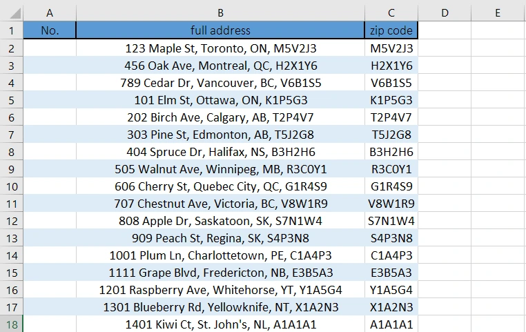
Fill Handle in Excel manages to discern a pattern based on the cells that already contain data and it automatically fills the other rows using that pattern. Let’s learn how to autofill row numbers in Excel with an example. Imagine you have a database like this:

• Enter the number ‘1’ in cell A2 and the number ‘2’ in cell A3.
• Select both cells (A2 and A3).
• A small square appears on the bottom right corner of the last cell.

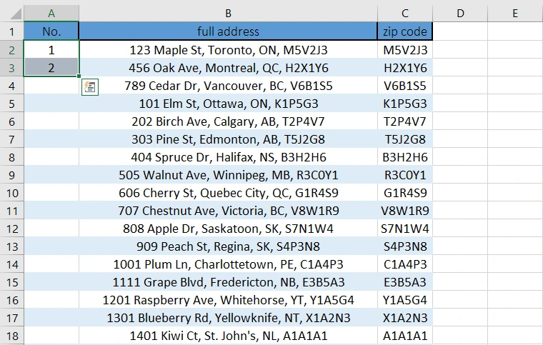
• Move the mouse cursor to that square. It will turn into a plus (+) icon.
• Double-click on the plus icon. It will automatically fill the rest of the column.

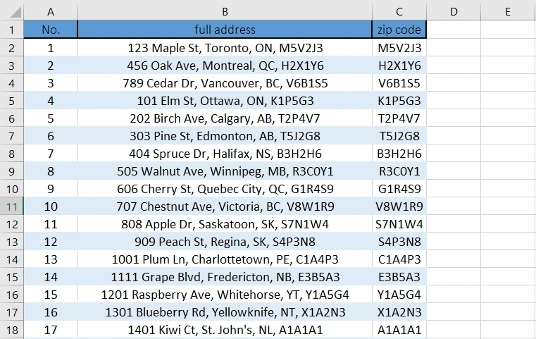
The fill handle recognizes the pattern of the data in the selected cells and fills the rest of the cells based on that pattern. In this case, the numbers in the cells are increasing by 1. So, it will continue filling the cells in the same manner—3, 4, 5, and so on.

• Please, note that if the adjacent column does not contain data, the double-click on the plus sign will not work. In that case, you have to click and hold the plus sign, and then drag down to fill the cells.

Enhance your software capabilities with our customizable Add-In Solutions, seamlessly integrating new features to meet your business needs.

If you’re working with data and want to go beyond numbering rows, check out our guide on how to add numbers in Excel, including cells and entire columns.

Customizing the Autofilled Row Numbers (Fill Series)

But how to autofill row numbers in Excel when you need a different starting number or an increment other than one? Well, autofill is flexible! Using the Fill Series function, you can easily customize the autofilled row numbers based on your requirements and the dataset features.

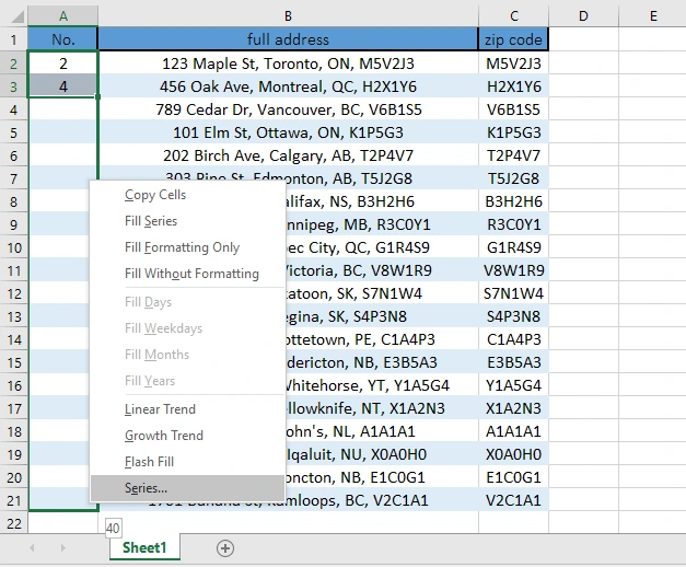
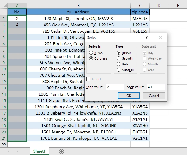
To access custom row numbering in Excel, right-click as you drag the Fill Handle and select “Series”. You will then see the series dialog box where you can change the step value, set a specific stop value, and change the type of series.

Imagine you want to number the rows with even values from 2 to 40. You should type 2 in the first row, 4 in the second row, and then drag and select series. In the dialog box, assign 2 to step value and 40 to stop value, and then click OK. Here is the result:

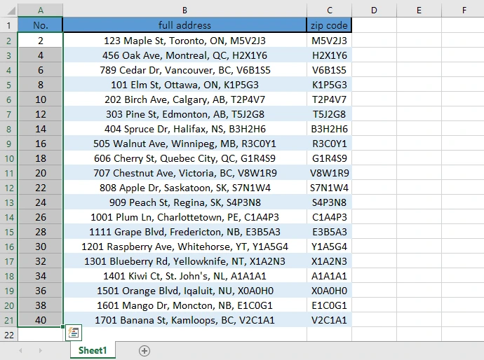
This option is particularly handy for specialized data entries or creating unique identifier systems. Moreover, you don’t need to drag the fill handle to your desired row as determining the stop value helps you fill all the rows as you wish!

Using Excel Functions for Row Numbers

In the Fill Handle method, the number assigned to rows is a static value. Meaning if you add or remove rows in your sheet, the assigned numbers do not change. Therefore, you will have to follow the steps again to update the row numbers to the correct values.  

This problem can be fixed using time-saving Excel techniques. You can use the ROW() function in Excel for numbering rows. In order to number the rows using this function, enter the formula below for the first row, and then copy it for the rest:

=ROW(A2) -1

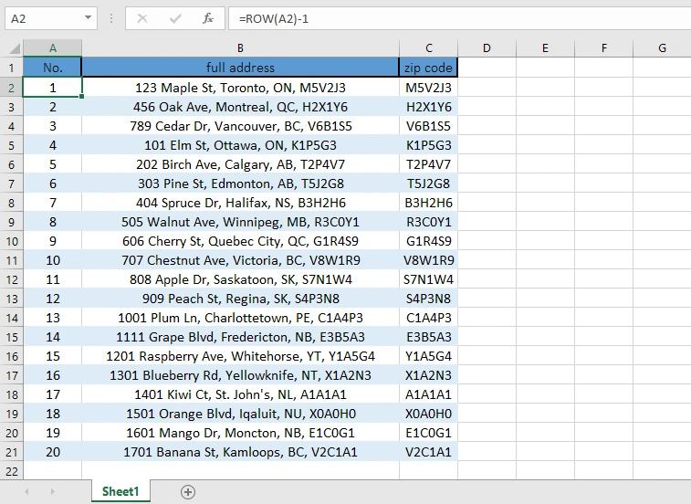
The ROW function shows the number of the current row. That’s why in this example, we subtracted 1 from the formula and wrote it as ROW () -1.  If your data starts from row five, you would have to write the formula as such: =ROW(A5)-4

The advantage of using this method for numbering rows is that when you remove or add new rows to the mix, you will not mess up the numbering. It will automatically adjust the row numbers based on the new information. Note that as soon as a row is deleted, the numbers adjust accordingly.

This method doesn’t take empty rows into account. It will still number rows even if they contain no data at all. You can use the formula below to hide the empty row numbers.

=IF(ISBLANK(B2),””,ROW()-1)

Autofilling Row Numbers in Large Datasets

In order to autofill large datasets in Excel, where dragging the fill handle doesn’t seem practical, a more efficient approach is needed. Let’s see how to autofill row numbers in Excel when working with large datasets:

• Enter ‘1’ in the first cell: Start by entering ‘1’ in the first row of the column where you want the numbers.
• Use the ROW function: In the cell below, instead of entering ‘2’, enter the formula =ROW()-1. This formula will return the row number of the cell.
• Copy the formula: Copy the formula in the second cell.
• Select the destination range: Click on the cell with the formula, then press Ctrl + Shift + Down Arrow to select the range down to the last row.
• Paste the formula: Press Ctrl + V to paste the formula. This will apply the ROW() formula to all selected cells, giving each cell the corresponding row number.

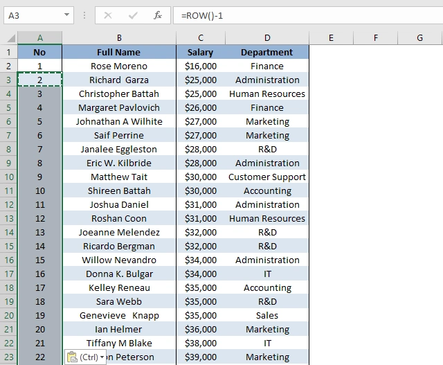
This approach should efficiently number the rows in large datasets without the need for dragging the fill handle.

Boost your productivity by getting a free consultation from Excel experts, and discover tailored solutions to optimize your data management and analysis.

Autofilling Row Numbers in Filtered or Sorted Data

You may need to number the Excel rows when your data is filtered or sorted. The key here is to ensure that the row numbering only reflects the visible rows. Using the SUBTOTAL function can be a clever way to autofill filtered data in Excel. Here’s a step-by-step guide with an example:

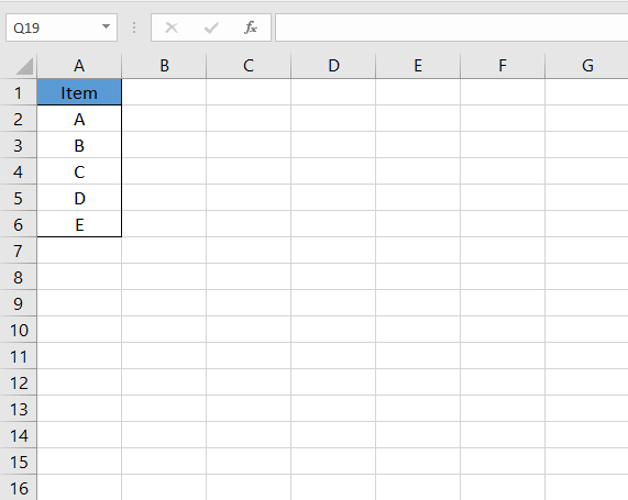
Imagine you have a dataset of 5 items (A, B, C, D, E) in Excel, and you want to autofill row numbers that adapt to sorting and filtering.

Step 1: Create Your Data

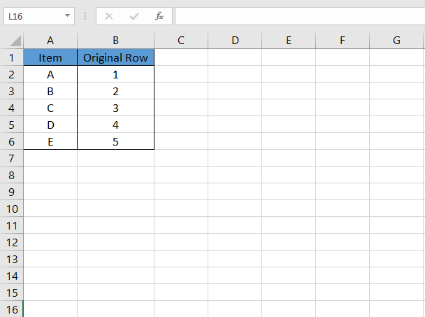
Add a Column for Static Row Numbers (Helper Column).

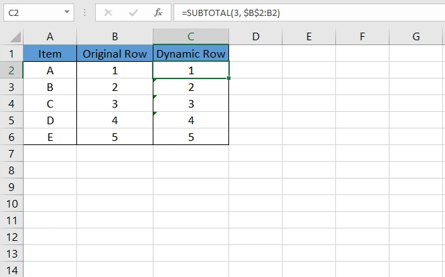
Step 2: Add a Dynamic Row Number Column

• Add Another Column for Dynamic Row Numbers.
• Enter the formula =SUBTOTAL(3, $B$2:B2) in cell C2.
• Drag this formula down from C2 to C6.

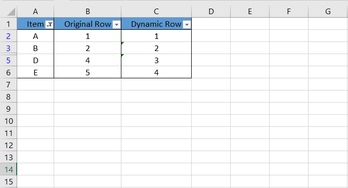
Step 3: Apply Filters or Sorting

For example, filter out item “C”.

Step 4: Observe the Row Numbers

• Column B (Original Row) remains unchanged, reflecting the initial order.
• Column C (Dynamic Row) changes based on visible rows.

Conditional Autofill for Row Numbers

Sometimes you don’t want to number all the rows and just need to number the ones that meet a certain criterion. In these situations, you can count on conditional autofill in Excel as a beneficial solution. To conditionally autofill row numbers based on specific criteria, you can use a combination of the IF function and row counting formulas.

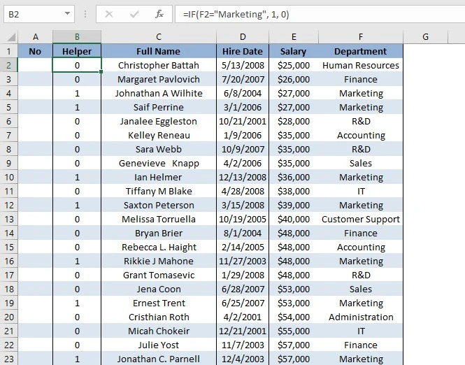
Conditional numbering is useful for scenarios like tracking specific types of data entries. Let’s see how to autofill row numbers in Excel when having certain criteria. Suppose you’re managing a table containing data about your employees and want to number the rows where employees work in the “Marketing” department. Here’s an adjusted approach:

In a new column (say Column B), use the formula =IF(F2=”Marketing”, 1, 0). This assigns ‘1’ to rows that meet your criteria and ‘0’ otherwise. Drag the formula down to fill the entire column.

In column A where you want your final numbers, use the formula =IF(B2=1, SUM($B$1:B2), “”). This formula sums the values of the helper column and provides a sequential count for rows that meet the criteria.

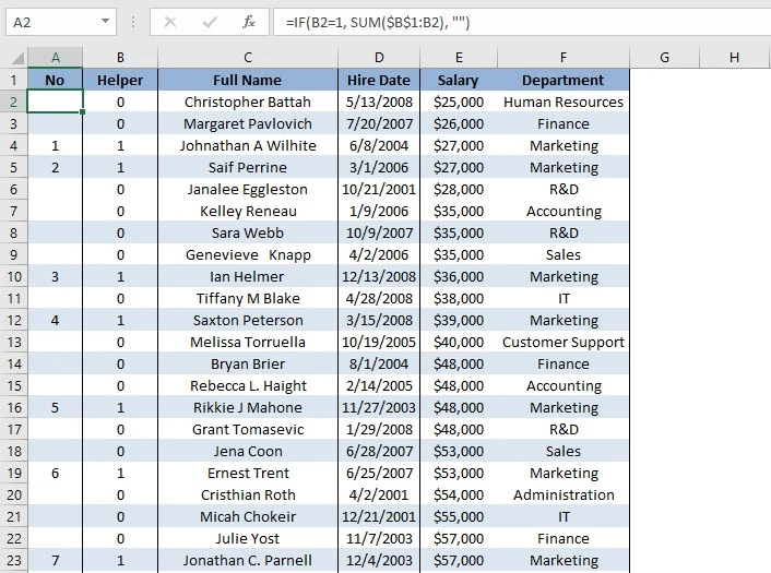
With this method, the numbering in Column A will start from 1 and increment sequentially for each row, maintaining row order in Excel.

Unlock valuable insights with our Data Visualization and Data Analytics Services, transforming complex data into clear, actionable strategies for informed decision-making.

If you’re looking for more advanced pasting techniques, such as using the Paste Special feature to control how your data is pasted, check out our guide on Operations with Paste Special in Excel.

Best Practices for Row Numbering in Excel

To maintain consistent and error-free row numbers, follow these best practices for Excel row numbering:

1. Automated Numbering: Use tools like the Fill Handle or functions like `ROW()` for automatic numbering to minimize manual errors and ensure consistency across large datasets.

2. Regular Data Verification: Check your numbering for any irregularities, such as missing numbers or duplicates regularly. This can significantly help you after sorting, filtering, or modifying the data.

3. Documenting Numbering Schemes in Excel: Keep a record of your numbering methodology, including any custom rules or formulas used. This documentation is crucial when sharing your Excel files with others or revising the dataset after some time.

4. Conditional Formatting for Error Detection: Implement conditional formatting rules in Excel to automatically highlight any anomalies in your numbering, like unexpected gaps or sequence jumps.

5. Regular Backups: Regularly save backup copies of your Excel files to prevent any accidental data loss or changes that might disrupt your numbering system.

6. Adapt Numbering to Data Changes: When adding, removing, or modifying rows, update your numbering scheme accordingly to maintain accuracy. For instance, if rows are deleted, ensure the numbering adjusts to fill in the gaps.

Conclusion

Autofilling row numbers in Excel is not just about saving time; it’s about enhancing the accuracy and efficiency of your data management. In this blog post, we explored how to autofill row numbers in Excel for data management, covering different situations and data types. Embrace this feature and watch as it transforms your Excel tasks, giving you more time to focus on what truly matters in your data analysis journey.

FAQs