How to Split Cells in Excel

Comfortable and satisfying as it is, working with Excel can sometimes be confusing. There sure have been times when you entered a lot of data in single cells under a column and decided later that all the information in those single cells better be divided into different cells under multiple columns. At times like this, you need to know how to split cells in Excel!

In this tutorial, we are going to explain three methods to split cells in Excel.

Splitting Cells Using Text to Column Feature

Suppose that you have a spreadsheet containing some information about a group of people, including first name, last name, and ID number and you want to put this information in separate cells.

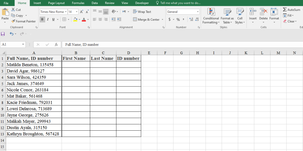
You can split these data following these steps:

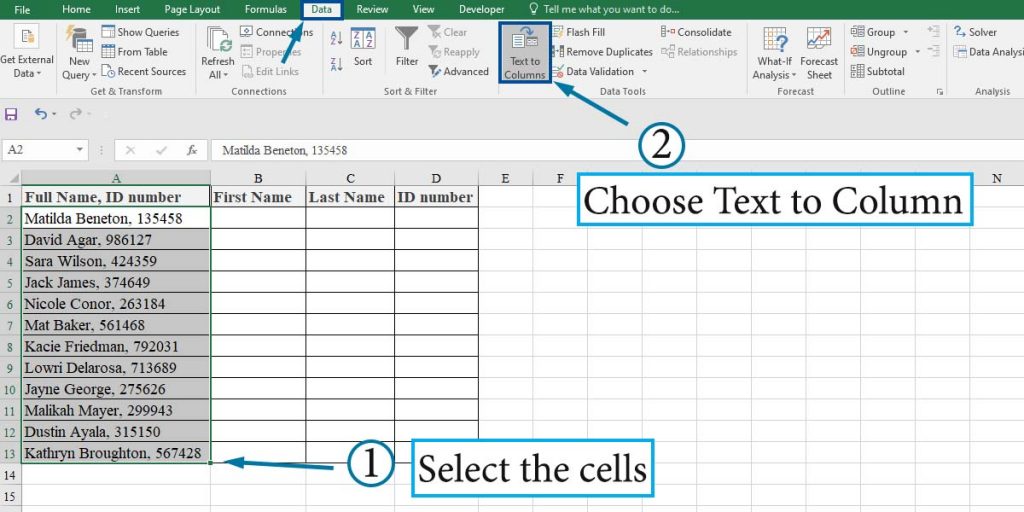
1. Select the cells you want to split the data.
2. Go to the Data tab and choose “Text to Column” from the Data Tools group.

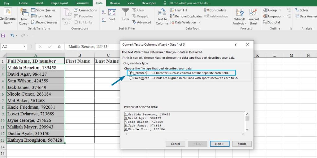
3. The “Convert text to column wizard” window will open. This part includes three steps:

• Step 1 of 3: At this step, you have 2 options: Delimited and Fixed Width. Choose the “Delimited” option, which is the character by which you specify to split cells and then click Next.

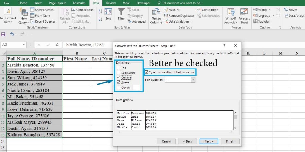
• Step 2 of 3: Since our data are separated by space and comma, you must choose both as delimiters and then click Next. Also, you’d better check the “Treat consecutive delimiters as one” box. You can see the result in the Data preview section.

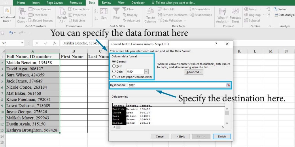
• Step 3of 3: At this stage, you can specify the data format and the data destination. Leave the data format as General. Change the destination to $B$2 by typing it or clicking on the icon and selecting a range on the spreadsheet. Having set the information, click Finish.

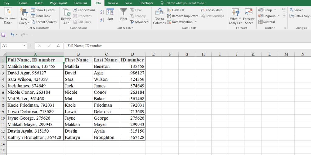
And here’s the result.

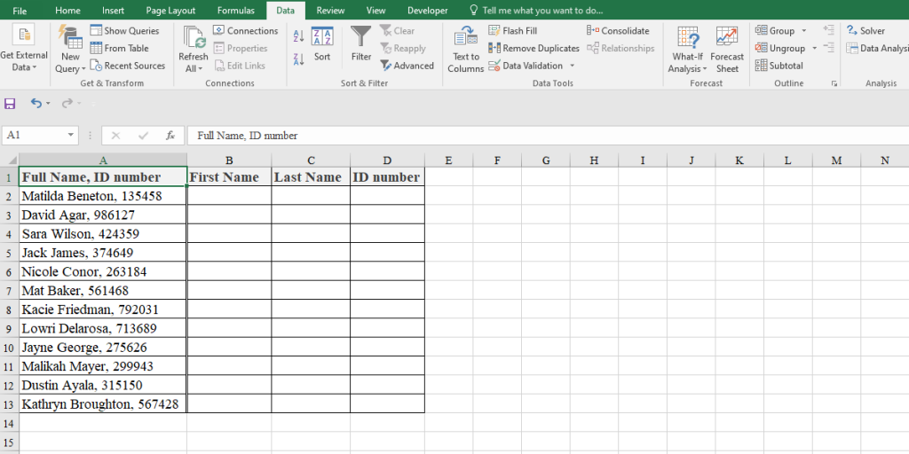
Note: If you leave the destination as default, Excel will keep the first column where it is and move the rest to the next columns.

 

 

Splitting Cells Using the Flash Fill Feature

Another easy way to split cells in Excel is using the flash fill option. To split cells in the previous example, we just need to write the part of the text that we want splitted in the desired cell, then use the flash fill feature.

Suppose that you want to extract the first names, last names, and ID numbers from the first column and put them in the next columns. All you need to do is to follow these steps:

• In Cell B2, type the corresponding first name (i.e., Matilda).
• Press “Ctrl+E,” which is the shortcut for the flash fill option.
• Do the same thing for the last names and ID numbers.

Note: If you don’t want to use shortcuts, you can go to the Data tab and click on Flash Fill from the Data Tools group.

https://youtu.be/GtM76UR2OZY

 

Splitting Cells Using Text Functions

The last method to split cells is using Excel text functions. Excel text functions work great when you want to split cells. You must know how to use these functions and how to combine them.

Here are the text functions that we can use to split cells in Excel:

•  LEFT: It extracts a specific number of characters from the left side of a string
• FIND: We use it to find a string inside another one. It returns the starting position of the sub-string as a number.
• RIGHT: It extracts a specific number of characters from the right side of a string.
• LEN: It returns the total number of characters in a text string.
• MID: It extracts a substring from a text string. It returns the number of characters starting from the position you specify.
• SUBSTITUTE: It replaces one or more text strings with another one.

Note: Excel SEARCH function does the same thing as the FIND function. The only difference is that the FIND function is case-sensitive, but the SEARCH function is not.

Now that we know the text functions we need, we can directly go to the examples.

Extracting the First Name

This example shows how to extract the first names from a list containing first names and last names.

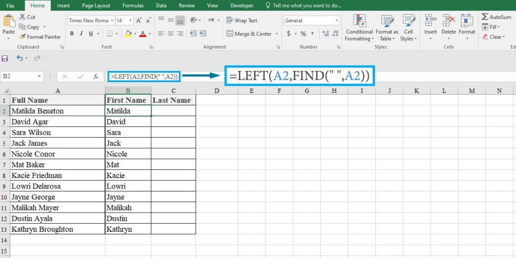
To extract the first names, we can use the combination of the LEFT function and the FIND function. To do so, we use the following formula:

=LEFT(A2,FIND(" ",A2))

In this formula, the FIND function finds the space character’s location as a number and gives it to the LEFT function to split the first name from cell A2.

Note: This formula works for the previous example too.

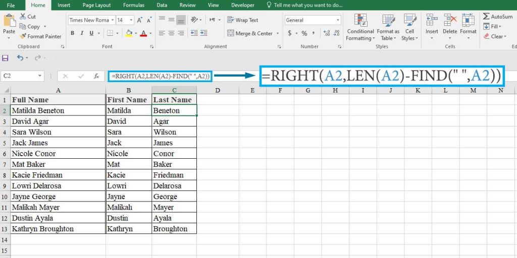
Extracting the Last Name

To extract the last names, we use a combination of the RIGHT, FIND, and LEN functions. To do so, we use the formula below:

=RIGHT(A2,LEN(A2)-FIND(" ",A2))

This formula locates the space character and splits the characters after it.

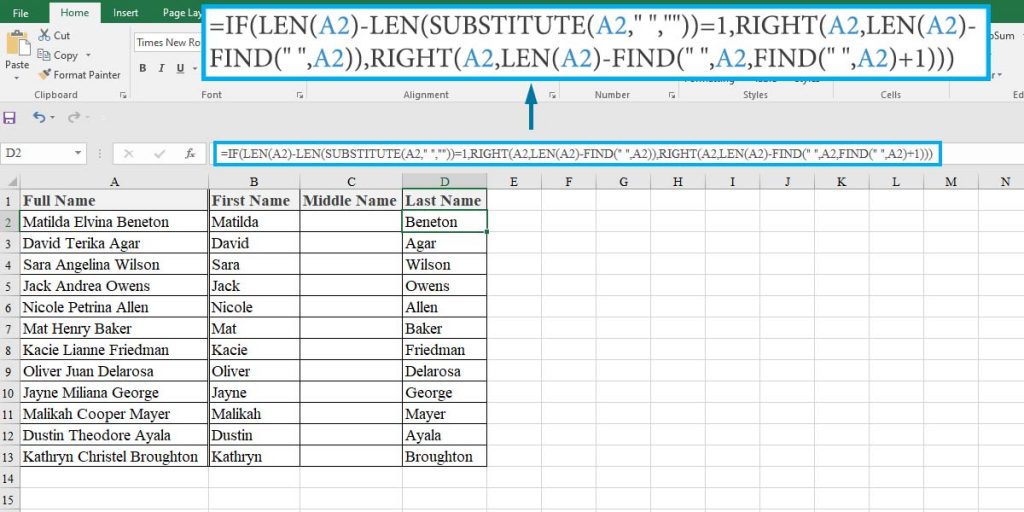
If our list includes middle names, we have to combine the above functions with IF and SUBSTITUTE functions. Look at the formula below:

=IF(LEN(A2)-LEN(SUBSTITUTE(A2," ",""))=1,RIGHT(A2,LEN(A2)-FIND(" ",A2)),RIGHT(A2,LEN(A2)-FIND(" ",A2,FIND(" ",A2)+1)))

In this formula, the IF function checks the existence of a middle name. The formula counts the number of the space characters; if there is only one, it uses the exact formula we introduced for extracting the last name before; if there are two spaces, it locates the second one and splits the next characters.

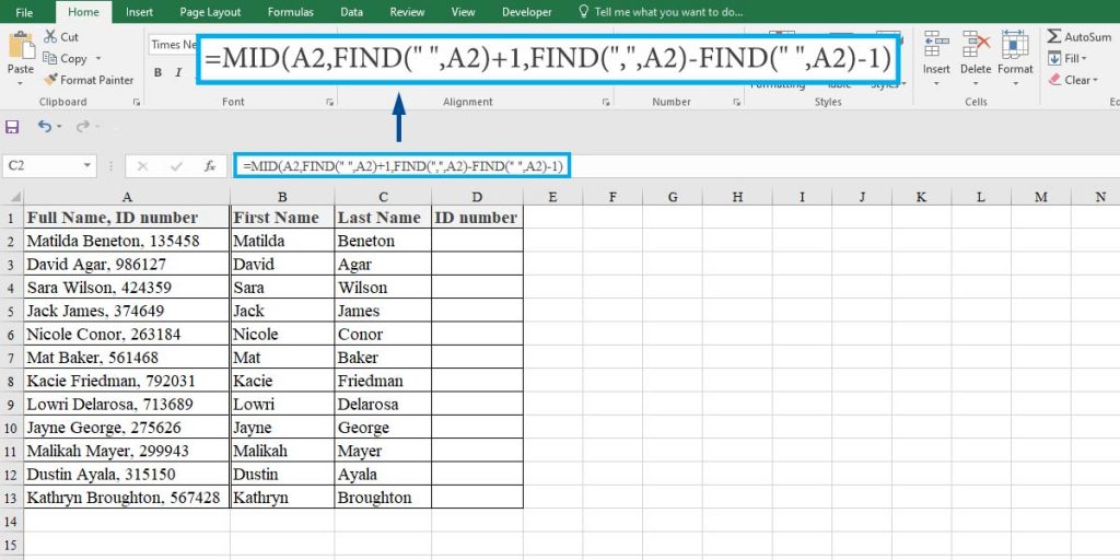
Now, what if we had the first example’s data and wanted to extract the last names? The answer is the combination of the MID and FIND functions as below:

=MID(A2,FIND(" ",A2)+1,FIND(",",A2)-FIND(" ",A2)-1)

Extracting the Middle Name

Sometimes, you have a list of names that include middle names, like the second example about the last names. To extract the middle name from a text, we combine the MID and SEARCH functions. Look at the following formula:

=MID(A2,SEARCH(" ",A2)+1,SEARCH(" ",A2,SEARCH(" ",A2)+1)-SEARCH(" ",A2))

In this formula, the MID function extracts the characters between the two spaces.

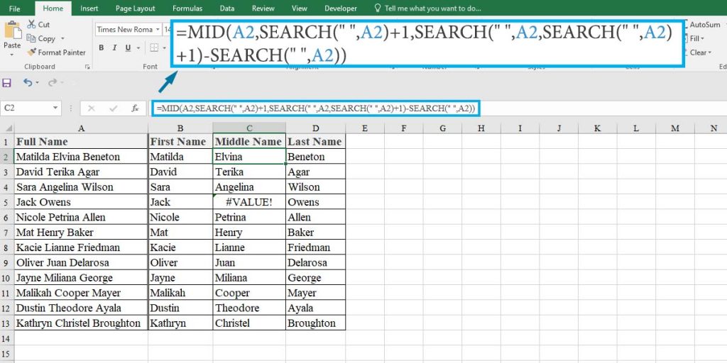
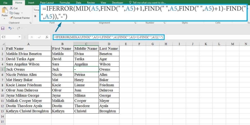
Note: If you enter the above formula for a text without a middle name, it returns the #VALUE error. To avoid this, you can use the IFERROR function. Look at the formula below:

 =IFERROR(MID(A5,FIND(" ",A5)+1,FIND(" ",A5,FIND(" ",A5)+1)-FIND(" ",A5)),"-")

Here, the text in cell A5 does not have a middle name, so the formula returns the “-” character. It’s obvious that if we use it for cell A2, it will give the middle name.

We have covered three simple methods to split cells in Excel. Now, you have a choice, so see which one you are more comfortable with and try that one out.

You can connect with us and ask our experts for your inquiries and get more Excel Support Service.

Reduce cost, accelerate tasks, and improve quality with Excel Consulting Service.