How To Subtract In Excel

How to subtract in Excel

Unlike the SUM function which has a predefined formula in Excel, subtraction in excel should usually be done manually. However, you can also write a macro for subtraction in Excel. But in this tutorial, we will tell you how to do it manually. There are several methods to subtract in Excel, which are as follow:

Subtract in Excel Manually 

Excel Subtraction: Method 1

The easiest method to subtract in Excel is to do it in the cell where you are writing the original number. To do so, you should first select the cell where you want to see the result of subtraction. Let’s say it’s A1. Then, start your formula with “=” and write the numbers you want to subtracts and finally press “Enter.” For example, it should be something like this:

=12-10 [Enter]

The result will be shown in the same cell (A1 will turn into the result which is number 2)

Empower your business with our Excel Programming and VBA Macro Development Services, tailored to automate tasks and unlock the full potential of your data management capabilities.

Excel Subtraction: Method 2

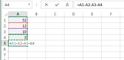
Sometimes you write the numbers in several cells and want to subtract their values. In this case, again, you should start by selecting the cell where you want to see the result. Suppose you want to subtract the values of A1 to A4 and see the result in A5. Select A5 and again start the formula with “=”. In the next step, select each cell manually and put a minus between them. For example, you should select A1 and then put a minus “-“, then select A2 and put “-“, and so on. Then press “Enter” to show the result in A5.

Excel Subtraction: Method 3

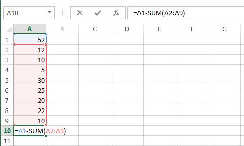
There is a question here: what if the subtracting cells are more than just a few. What if we want to subtract the values of A1 to A20? It will not be that easy to select each cell one by one. There is a solution to this case too. You should know which cells you want to subtract from which value. For example, do you want to subtract A2 to A19 from A1? If it’s the case, you can first SUM A2 to A19 in another cell (for example A20). Then subtract A20 from A1 in another cell. 

However, you can also do all these functions in one formula. First, select the cell where you want to see the result (for example A21), then like always, start your formula with “=”. Select the cell from which the subtraction should be done. In this example, it’s A1. Next, write “-“, and proceed with the formula with the SUM function. It should be something like this: 

=A1-SUM (A2:A19) 

You can either write the formula yourself or just do this by selecting the cells. 

Subtracting in Excel: Method 4

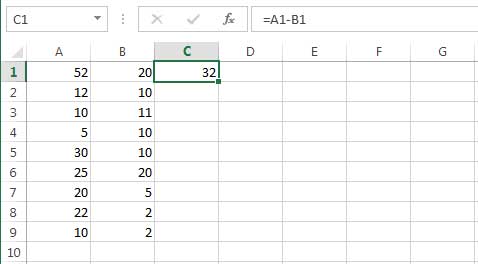
If you have two columns and need to subtract the value of column B from column A, you won’t need to write the formula each time. You just need to do it once and copy the formula for the rest. First, select C1 cell, and subtract B1 from A1. (the formula is =A1-B1)

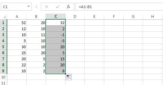
Next, put the cursor on the lower right corner of C1. It will change to a black + sign. You can either select and drag it to C10, or double click on the sign and all the other cells will be filled with the subtract values.

Subtracting in Excel: Method 5

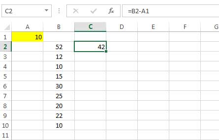
If you want to subtract the same number from all the cells, you should first put the number in one cell. Suppose the number is 10. So we select cell A1 and write 10. (In this example we write the numbers in a column  and want to see the results in column C.) 

Next, select C2, write “=” then select (B2-A1). The result will be 42.

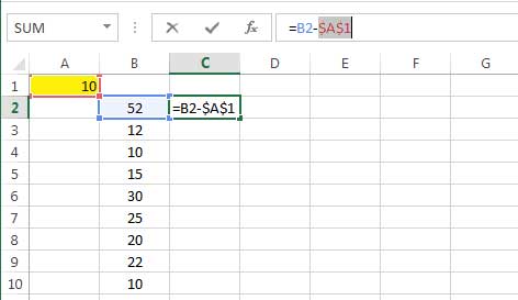
We want to do the same for other cells without having to write the formula one by one. In this case, you should fix the cell from which the subtraction is going to be performed. In this example, it’s A1. To fix A1 in the formula, you should select the formula in cell C2 and put the cursor behind A1 then press F4 on the keyboard. Two $ signs will be shown before and after A1 in the formula which indicates it’s been fixed.

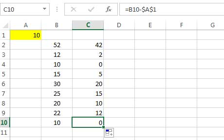
Now you can easily double click on the lower right corner of C2 and see the result. 

But what will happen if we don’t fix the cell? Check the picture below:

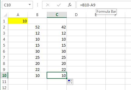
See the formula written in “Formula Bar.” If you don’t fix the cell, by dragging or double-clicking on the first cell you won’t see any change because the cell number will change too. As you can see, there is no value in A2 to A9; therefore, you won’t see any change. 

Boost your productivity by getting a free consultation from Excel experts, and discover tailored solutions to optimize your data management and analysis.

How to Subtract Date and Time

If your data have a Date format, you can subtract the start date from the end date to see the result or use the DATE or DATEVALUE functions:

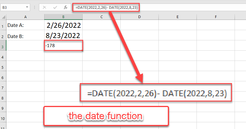
The DATE function syntax:

=DATE(year, month, day)

Example:

Date A: 2022/2/26

Date B: 2022/8/23

=DATE(2022,2,26)- DATE(2022,8,23)

If your data contains a date in a text format, you can use the DATEVALUE function to convert the date to a number. The DATEVALUE function syntax is:

=DATEVALUE(date_text)

Example:

Date A: 2022/2/26

Date B: 2022/8/23s

=DATEVALUE(“2/26/2022”)-DATEVALUE(“8/23/2022”)

=DATEVALUE(“26-FEB”)-DATEVALUE(“23-AUG”)

=DATEVALUE(“2022/02/26 “)-DATEVALUE(“2022/08/03”)

=DATEVALUE(“2022-FEB-26 “)-DATEVALUE(“2022-AUG-03”)

The date should be between January 1, 1900, and December 31, 9999.

If your data values are defined as a Time format, you can subtract them too. Here, the point is to change the formula cell format to the Time format.

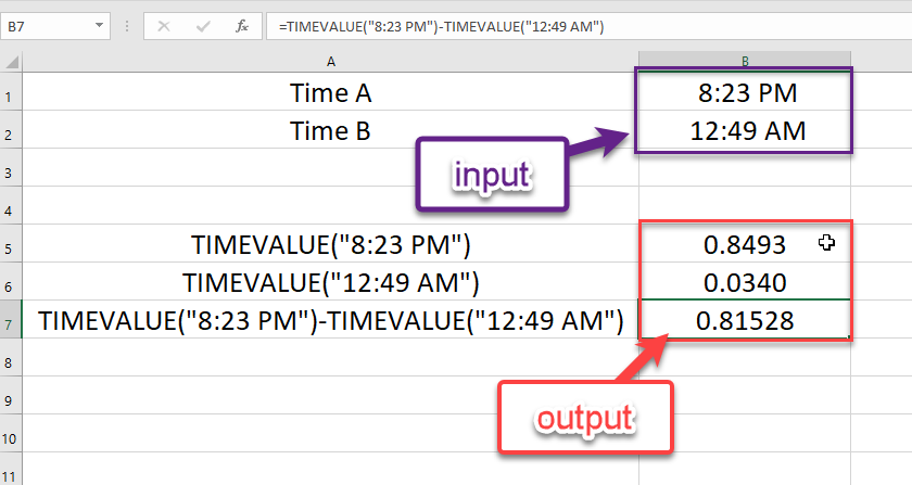
Also, you can use the TIMEVALUE function to convert a time_text into a suitable Excel time.

. The TIMEVALUE function syntax is:

=TIMEVALUE(time_text)

Example:

Time A: 8:23 PM

Time B: 12:49 AM

=TIMEVALUE(“8:23 PM”)-TIMEVALUE(“12:49 AM”)

Enhance your software capabilities with our customizable Add-In Solutions, seamlessly integrating new features to meet your business needs.

How to Subtract Matrix in Excel

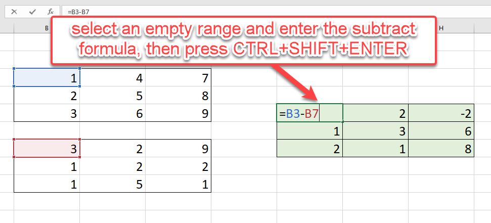
If you have matrixes as your data set, you can subtract the data only by one formula. So, follow these steps:

1.  Select an empty range based on the matrixes size.
2.  Enter the subtract formula:

=(the first matrix rang, the second matrix range, …)

3.  Press CTRL+SHIFT+ENTER.

Bottom Line 

By learning the different methods to subtract in Excel, you can easily do this function. It’s as easy as writing the numbers in different cells or writing a formula in the Excel formula bar. You can follow the method that is easier for you to remember. However, if you have an Excel sheet with lots of data, you may need to follow an advanced method of subtraction in Excel.