How to Wrap Text in Excel

In spreadsheet software like Microsoft Excel, which consists of several cells, sometimes you may need to have more room to display long texts on multiple lines. This is mostly useful when you are making a form in Excel. Wrap Text is a feature in Excel that helps you reach this result. You can wrap text in one or more Excel cells. In this post, we will explain to you how to wrap text manually and automatically.

How to Wrap Text in Excel Automatically?

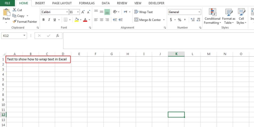
1. Select a cell and write your content (in our example, we selected cell A1). As you can see in Figure 1, the cell’s content A1 is too long and has taken the place of other cells. 

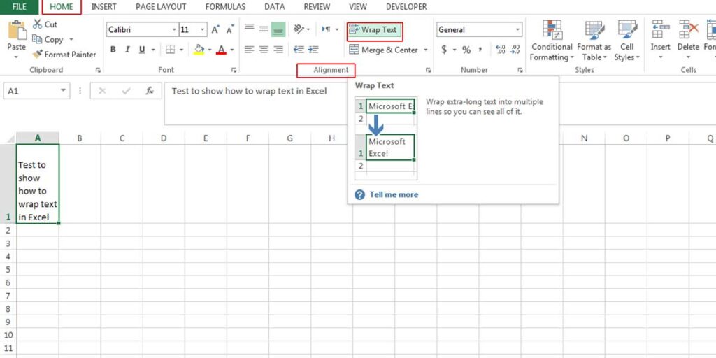
2. Select the cell (A1), go to the Home > Alignment section, and click on Wrap Text. You will see the following result.

Enhance your productivity and efficiency with our comprehensive Excel Automation Services, designed to simplify complex tasks and save you valuable time.

Wrap Text via Format Cells 

There is another method for using this feature in Excel. It’s as simple as the first method. 

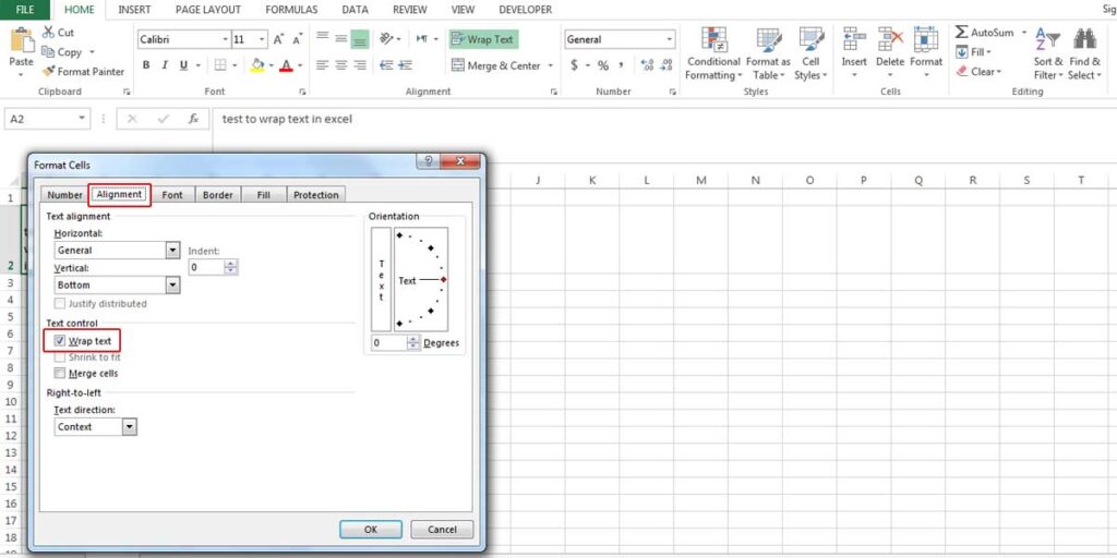
1. Right-click on the cell where you want to wrap text and select “Format Cells.”
2. In the Alignment tab, put a checkmark behind Wrap text. 

As you can see, it’s very simple. You can wrap text in Excel only in two steps. Now it is time to make some changes in the format of the cell to make it more clear and visible. 

How to Modify the Format of the Cell?

There are multiple options to modify the format of the wrapped cell. 

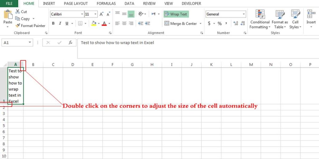
1. If you want to fit the cell’s height and width to your content, double click on the row header (in this example, it’s row 1) to automatically adjust the row height. You can do the same to the cell’s width by double-clicking on the corner of the cell (Cell A) to adjust the cell’s width. However, normally, Excel wraps the text with the column width and changes the height. If you double click on the right border of the column header before wrapping text, it fits the cell’s width to the text.

2. You can manually modify the cell’s width or height by clicking on the right border and dragging the separator to change the column width.
3. You can also do the same for changing the row height, or adjusting the height by double-clicking on the row heading’s bottom border.
4. It is also possible to set a defined size for the cell. In this case, you may not be able to change the size of the cell by other methods. 

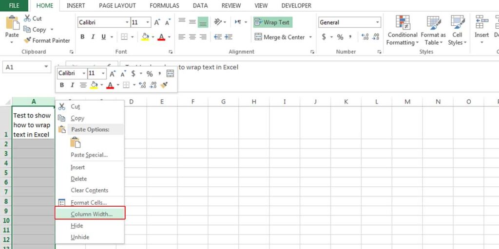
• To define a size for column width, right-click on the column header and choose “Column Width” then, set a size. 
• To define a size for row height, right-click on the row header and choose “Row Height” and set size. 

Boost your productivity by getting a free consultation from Excel experts, and discover tailored solutions to optimize your data management and analysis.

How to Insert a Break Line Manually?

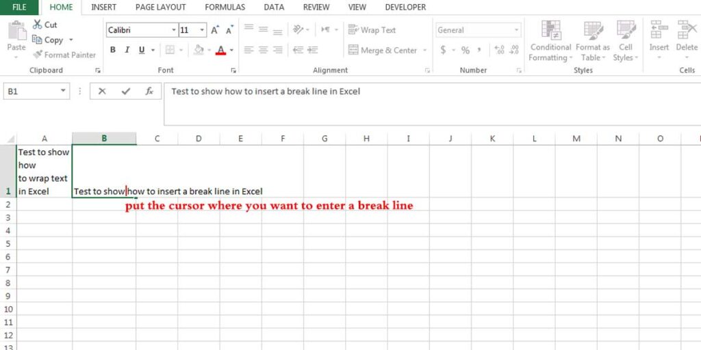
1. Double-click on the cell and put the cursor where you want to enter a line to break. In our example, we want to enter a break line after the word “Show.”

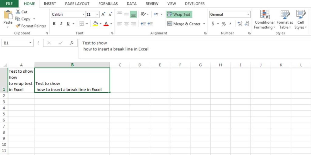
2. Press Alt+ Enter. You can see the rest of the sentence is moved to the next line. 

Bottom Line 

Wrapping text in Excel is so useful for making different tables and forms, especially when you are restricted to a specific size, such as A4 or letter. It is possible to adjust the size of cells based on your preferences. And you can also clear up your sentences by entering break lines manually. These two methods can help you make better reports and forms in Excel.