Excel ADDRESS Function for Dynamic References
In Excel, it’s essential to be precise and adaptable in your tasks. The Excel ADDRESS function is a valuable tool for achieving these qualities. Whether you’re working on tasks that involve creating dynamic references or manipulating data, having a good grasp of how to use the ADDRESS function effectively can significantly improve your Excel skills.
In this guide, we will thoroughly explore the ADDRESS function in Excel. We’ll cover its syntax, how to use it, advanced techniques, and best practices. By the end of this guide, you’ll have the knowledge and skills to make the most of ADDRESS in your Excel tasks.
What Is the Excel ADDRESS Function?
The ADDRESS function is a built-in function in spreadsheet software like Microsoft Excel and Google Sheets which is categorized under the Lookup and Reference functions.
The ADDRESS function mainly aims to create a text representation of a cell address based on the input row and column numbers. It can be helpful in various scenarios, such as when you want to create dynamic formulas that reference cells based on certain conditions or when you need to generate cell addresses for use in other functions or formulas. The ADDRESS function is typically used in combination with SUBSTITUTE, ROW, COLUMN, ROWS, INDIRECT, MATCH, and INDEX functions. Let’s dive into a detailed explanation of how the ADDRESS function works.
Boost your productivity by getting a free consultation from Excel experts, and discover tailored solutions to optimize your data management and analysis.
Syntax and Arguments
ADDRESS(row_num, column_num, [abs_num], [a1], [sheet])
| Argument | Type | Required/Optional | Explanation |
| row_num | Numeric | Required | Specifies the row number you want to include in the cell address. It can be any positive integer or a reference to a cell containing a row number. |
| column_num | Numeric | Required | Specifies the column number you want to include in the cell address. It can be any positive integer or a reference to a cell containing a column number. |
| abs_num | Numeric | Optional | Specifies the type of cell reference to return. 1 or omitted: Absolute, e.g. $A$1 2: Absolute row; relative column, e.g. $A1 3: Relative row; absolute column, e.g. A$1 4: Relative, e.g. A1 |
| a1 | Logical | Optional | Specifies A1 or R1C1 reference style 1 or True or omitted: A1 style, e.g. C3 0 or False: R1C1 style, e.g. R3C7 |
| sheet_text | Text | Optional | Specifies the name or index of the sheet address. If omitted, it refers to the current sheet, e.g. sheet2!$G3 |
Basic Usage Examples
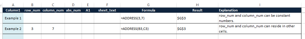
Here is a comprehensive list of basic usage examples of the ADDRESS function to demonstrate how to generate cell references dynamically.
- Using only required arguments.
- Finding addresses in the same sheet

- Finding addresses in another sheet

- Finding addresses in another workbook

Advanced Techniques – Using ADDRESS with other Excel Functions
The ADDRESS function in Excel and other spreadsheet software is quite versatile and can be used for more advanced tasks beyond basic cell referencing. Here are some advanced uses of the ADDRESS function.
Finding the Last Item in a Dynamic Range
When it comes to combining the ADDRESS function with other Excel functions, INDIRECT is the most common one. We can use the ADDRESS function nested in the INDIRECT function to find the value of the last item in a table.
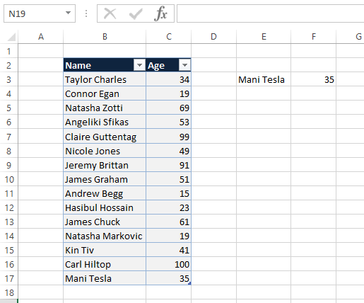
In the following screenshot, we have an Excel table containing the names and ages of some people. Although we can select the table and create a named range for each column, we prefer to continue with structured referencing using the table name which is tbl_ages_last in our case.

Use the following formula to find the last name in the table.
| Formula | Result |
| =INDIRECT(ADDRESS(ROW(tbl_ages_last[Name])+ROWS(tbl_ages_last[Name])-1,COLUMN(tbl_ages_last[Name]))) | Carl Hiltop |
Drag the formula to the right and you will have the last age effortlessly.

Now if we add a new row, the table and the table will pick up the new values automatically and the formula will handle all changes accordingly.
If you are interested, take a look at the following picture for a detailed breakdown of the formula we used in this section.

| Warning: INDIRECT is a volatile function. Cells with volatile functions, together with all dependents are reevaluated per every recalculation. For this reason, excessive use of volatile functions, especially when your data is large, can make recalculation times slow. Use them sparingly. |
Enhance your productivity and efficiency with our comprehensive Excel Automation Services, designed to simplify complex tasks and save you valuable time.
Calculations on the n Last Rows of a Dynamic Range
In this section, we show you how to perform calculations on the n last rows of a range. We will calculate the max, min, sum, and average of n (which is set through a dropdown list) last values of a table. With this technique, the final result will instantly react to the dynamics of the range.
Let’s start with a small dataset and create a table using this data. Creating a table is the key to making the final result adaptive to changes in the input range.

Use the following formulas to find the max, min, sum, and average of the n last ages in the table.
| Formula | Result | Description |
| =MAX(INDIRECT(ADDRESS(ROW(tbl_ages_last)+ROWS(tbl_ages_last)-n,COLUMN(tbl_ages_last[Age]))&”:”&ADDRESS(ROW(tbl_ages_last)+ROWS(tbl_ages_last)-1,COLUMN(tbl_ages_last[Age])))) | 100(for n=6) | Maximum of the last n ages |
| =MIN(INDIRECT(ADDRESS(ROW(tbl_ages_last)+ROWS(tbl_ages_last)-n,COLUMN(tbl_ages_last[Age]))&”:”&ADDRESS(ROW(tbl_ages_last)+ROWS(tbl_ages_last)-1,COLUMN(tbl_ages_last[Age])))) | 19(for n=6) | Minimum of the last n ages |
| =SUM(INDIRECT(ADDRESS(ROW(tbl_ages_last)+ROWS(tbl_ages_last)-n,COLUMN(tbl_ages_last[Age]))&”:”&ADDRESS(ROW(tbl_ages_last)+ROWS(tbl_ages_last)-1,COLUMN(tbl_ages_last[Age])))) | 279(for n=6) | Sum of the last n ages |
| =AVERAGE(INDIRECT(ADDRESS(ROW(tbl_ages_last)+ROWS(tbl_ages_last)-n,COLUMN(tbl_ages_last[Age]))&”:”&ADDRESS(ROW(tbl_ages_last)+ROWS(tbl_ages_last)-1,COLUMN(tbl_ages_last[Age])))) | 46.5(for n=6) | Average of the last n ages |
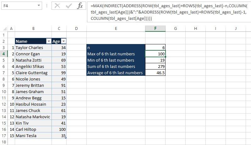
If you are interested, take a look at the following picture for a detailed breakdown of the formula we used to calculate MAX in this section.

| Warning: INDIRECT is a volatile function. Cells with volatile functions, together with all dependents are reevaluated per every recalculation. For this reason, excessive use of volatile functions, especially when your data is large, can make recalculation times slow. Use them sparingly. |
Convert a Column Number to a Letter
You can use the ADDRESS function nested in SUBSTITUTE to get the column letter using a column number.
You can use the column number as a constant number in the formula.
| Formula | Result | Description |
| =SUBSTITUTE(ADDRESS(1,37,4),”1″,””) | AK | Using a constant number as the column number |

Or you may use the column number as a numeric value in another cell.
| Formula | Result | Description |
| =SUBSTITUTE(ADDRESS(1,E2,4),”1″,””) | AK | Using the value of another cell as the column number |

Had you have wanted to get the letter of the current column, type the following formula in the cell you want to find its column letter.
| Formula | Result | Description |
| =SUBSTITUTE(ADDRESS(1,COLUMN(),4),”1″,””) | E | Letter of the current column |

If you are interested, take a look at the following picture for a detailed breakdown of the formula we used for the last case.

Find the Address of a Named Range or Table
In this section, we investigate how to use the ADDRESS function to find the address of a named range or table.
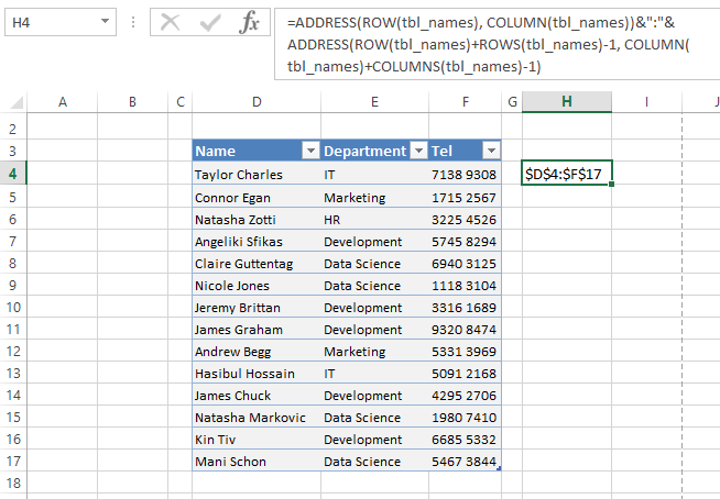
Let’s assume we have an Excel file like the following picture in which we have created a table from data. This gives us a benefit over a named range. With a table, if you add more rows or columns to the data, the formula will pick up the new values automatically.

Enter the following formulas in a blank cell to find the address of the table/range you have created.
| Formula | Result |
| =ADDRESS(ROW(tbl_names), COLUMN(tbl_names))&”:”&ADDRESS(ROW(tbl_names)+ROWS(tbl_names)-1, COLUMN(tbl_names)+COLUMNS(tbl_names)-1) | $B$3:$D$15 |
If you are interested, take a look at the following picture for a detailed breakdown of this formula.

Add some data to the table or change its position, you can see that the formula is robust and adaptive to this change.
Get the Address of the Max and Min Values in a Range
In this section, we will show how to find the address of the highest and lowest value in a range that is robust to any possible change in the position and size of the range.
Let’s assume we have an Excel file like the following picture. We need the addresses of the maximum and minimum age, which in our case are C7 and C11 respectively.
In the first step, we create a table from data in our file. This is the key to making the formula robust to change in the number of rows and columns.

Enter the following formulas in empty cells to find the addresses of min and max values in the table you created in the previous step.
| Formula | Result | Description |
| =ADDRESS(MATCH(MAX(tbl_ages),tbl_ages[Age],0)+ROW(tbl_ages)-1, COLUMN(tbl_ages[Age])) | $C$7 | Address of the maximum age |
| =ADDRESS(MATCH(MIN(tbl_ages),tbl_ages[Age],0)+ROW(tbl_ages)-1, COLUMN(tbl_ages[Age])) | $C$11 | Address of the minimum age |
If you are interested, take a look at the following picture for a detailed breakdown of the formula for maximum value.

Add some data to the table or change its position, you can see that the formula is robust and adaptive to this change.

This helpful guide provides step-by-step instructions for those looking to parse addresses in Excel using VBA macros: ‘How To Parse An Address In Excel By Macro/VBA.‘
Tips and Best Practices
Here are some tips and best practices for efficiently using the ADDRESS function in Excel, as well as maintaining clarity and readability in your formulas:
- Understand the Purpose: Ensure you understand when and why to use the ADDRESS function. It’s most helpful to generate cell references based on row and column numbers dynamically.
- Use Relative and Absolute References Wisely: Consider the `[abs_num]` argument. Decide whether you need relative or absolute references for rows, columns, or both. Choosing the right combination is crucial for the behavior of your formulas.
- Leverage the A1 vs. R1C1 Styles: Depending on your preference and specific needs, you can choose between the A1 reference style (e.g., “A1”) and the R1C1 reference style (e.g., “R1C1”) using the `[a1]` argument.
- Consider Naming Conventions: When using the ADDRESS function extensively, consider adopting naming conventions for your cell references to enhance clarity and organization.
- Combine with other Functions: The ADDRESS function is often combined with other functions like INDIRECT to create dynamic and powerful formulas.
- Some of the functions we typically use in combination with Address are volatile. Be mindful when using these functions as they can affect your performance.
- Break Down Complex Formulas: If a formula becomes too complex, break it into smaller, manageable parts using intermediate cells to store intermediate results.
- Comments: Insert comments in your formulas (via the “Insert Comment” option) to explain complex or non-obvious parts of your calculations. These comments are valuable for you and others working with your spreadsheet.
- Consistent Formatting: Keep consistent formatting throughout your workbook. Use the same style for headings, cell colors, and fonts to maintain a cohesive and professional appearance.
- Error Handling: Incorporate error handling in your formulas. Use functions like IFERROR or IF(ISERROR) to catch and handle errors gracefully.
- Documentation: Maintain documentation for your spreadsheet, especially if it’s complex or used by multiple people.
- Testing: Always test your formulas thoroughly with various scenarios and datasets to ensure they work as expected. Debugging complex formulas can be challenging, so testing is crucial.
- Version Control: If multiple people collaborate on the same spreadsheet, use version control tools or strategies to track changes and maintain a history of revisions.
- Consistency: Be consistent in your naming conventions, formatting, and organization. A consistent approach across your workbook enhances its overall clarity and readability.
Common Pitfalls and Troubleshooting
Users may encounter common mistakes or pitfalls when using the Excel ADDRESS function. Here are some of these issues, along with explanations on how to handle errors and troubleshoot them:
Common Pitfalls
- Incorrect Arguments: Providing incorrect or invalid arguments can lead to errors. Ensure that the `row_num` and `column_num` arguments are valid integers or references. Check that the `[abs_num]` argument is one of the allowed values (1, 2, 3, or 4). Make sure the `[a1]` argument is set to TRUE or FALSE.
- Misuse of Absolute and Relative References: Misusing the `[abs_num]` argument can result in incorrect cell references. Based on your formula’s requirements, understand when to use absolute or relative references for rows and columns.
- Lack of Error Handling: If the ADDRESS function is used within a larger formula or in a dynamic context where the referenced cell doesn’t exist, it can return an error (e.g., #REF!). Not handling these errors can lead to unexpected issues in your spreadsheet.
- Incorrect Sheet References: If you’re referencing cells in another sheet using the `[sheet]` argument, ensure that the sheet name or index is correct. Mistyping the sheet name or providing an invalid index can cause errors.
Handling Errors and Edge Cases
- Error Handling with IFERROR: To handle errors gracefully, wrap your ADDRESS function or any formula using it with the IFERROR function. For example:
- IFERROR(ADDRESS(3, 2), “Error: Invalid Reference”)
- This will display a custom error message (“Error: Invalid Reference”) when the ADDRESS function encounters an error.
- Avoid Circular References: Be cautious when using ADDRESS inside a formula that could result in circular references. Excel will display a circular reference warning, and your formula may not work as expected.
Troubleshooting and Fixes
- Check Argument Values: Double-check the values of your `row_num`, `column_num`, and other arguments. Ensure they are valid and appropriate for your formula.
- Test in Isolation: When encountering issues, break down your formula and test the ADDRESS function in isolation to identify where the problem lies. Once you’ve isolated the issue, you can address it more effectively.
- Evaluate Formula (Formula Auditing): Use Excel’s formula auditing tools to evaluate and trace precedents and dependents. This can help you identify errors and understand how formulas are interconnected.
- Review Sheet References: If you’re referencing another sheet, make sure the sheet name is spelled correctly and that it exists in your workbook. Check for typos and verify the sheet index if you’re using an index number.
- Inspect Cell References: If your formula uses dynamic references generated by ADDRESS, verify that these references point to the correct cells by clicking on the cell containing the formula and checking the highlighted cells in the worksheet.
- Check for Circular References: If you suspect a circular reference issue, navigate to the “Formulas” tab in Excel and use the “Error Checking” feature to locate and address circular references.
- Use the Excel Help Function: If you need help using the Excel ADDRESS function or any Excel function, use Excel’s built-in Help function (press F1) to access detailed documentation and examples.
Conclusion
The Excel ADDRESS function is a versatile tool to dynamically generate cell references based on row and column numbers. It’s used for:
- Creating cell references in A1 or R1C1 styles.
- Building dynamic named ranges for flexible data handling.
- Enabling advanced tasks like custom references and lookup formulas.
Best practices include error handling and clear formula organization. Beware of common pitfalls and use Excel’s auditing tools for troubleshooting. In summary, ADDRESS enhances Excel’s capabilities for automation and data analysis.
FAQs
The main difference between A1-style and R1C1-style references in the ADDRESS function is how the row and column numbers are represented.
In A1-style references, the row number is represented by a number, and the column number is represented by the column letter. For example, the cell address A1 refers to the cell in the first row and column.
In R1C1-style references, both the row and column numbers are represented by numbers. For example, the cell address R1C1 refers to the cell in the first row and column.
The default reference style in Excel is A1-style. However, you can change the reference style to R1C1 by going to File > Options > Formulas and selecting the R1C1 reference style check box.
The ADDRESS function can return either A1-style or R1C1-style references, depending on the value of the reference_style argument. If the reference_style argument is omitted or set to 4, the function will return an A1-style reference. If the reference_style argument is set to 5, the function will return an R1C1-style reference.
You can combine the Excel ADDRESS function and INDIRECT functions to perform complex tasks. For instance, to dynamically reference a cell in the same column as the currently selected cell and in the first row, you can use this formula:
=INDIRECT(ADDRESS(1, COLUMN(), 4))
In this formula, INDIRECT retrieves the value of the addressed cell.
This example showcases how you can harness ADDRESS and INDIRECT for various Excel tasks. With some creativity, these functions can handle a wide range of operations.
To handle situations where you need to reference cells in other worksheets using the ADDRESS function, you can use the sheet_name argument. The sheet_name argument is an optional argument that specifies the worksheet’s name containing the cell. If this argument is omitted, the function assumes the cell is on the active sheet.
For example, the following formula returns the address of the cell that is two rows down and three columns to the right of cell A1 on the worksheet named “Sheet2”:
=ADDRESS(2, 3, , “Sheet2”)
You can also use the sheet_name argument to reference cells in other workbooks. You must enclose the worksheet name in double quotation marks to do this. For example, the following formula returns the address of the cell that is two rows down and three columns to the right of cell A1 on the worksheet named “Sales” in the workbook named “MyWorkbook.xlsx”:
=ADDRESS(2, 3, , “‘MyWorkbook.xlsx’!Sheet2”)
Our experts will be glad to help you, If this article didn’t answer your questions. ASK NOW
We believe this content can enhance our services. Yet, it’s awaiting comprehensive review. Your suggestions for improvement are invaluable. Kindly report any issue or suggestion using the “Report an issue” button below. We value your input.


