10 Useful Functions for Data Analytics on Excel

 

Data Analytics Excel Functions

Excel is an excellent tool for data analysts because they can carry out different operations on this application. As a data analyst, some functions are more helpful for your job. Here is a list of Excel’s ten most useful functions for data analytics.

 

Which Functions Do Data Analysts Need to Learn? 

Sort and Filter

Sorting data is an inseparable part of data analytics, especially if you work on a table with vast data. You can sort data alphabetically, ascending or descending. Therefore, you can easily sort the list of data about customers’ names, or figure out which month you had higher sales.

The method is pretty simple:

1.  You only need to select the data you want to sort. 
2. And right-click on the selection.
3. Then select any of the options under  “Sort.” 

Please note that you need to select the whole table so that when you sort the data in one column, the rest of the table changes according to the sorted data.

You can also use Filters for sorting data in Excel. In this method, you should select the row on top of the table, which is normally the topic. Right-click and select one of the options under the “Filter.” Now you can sort data based on different values, even based on colours. You can also narrow down your list to the values you select from the list. For example, you can only see the red columns or specify an exact value. Filtering is a handy method when you have large data. 

IF Formulas

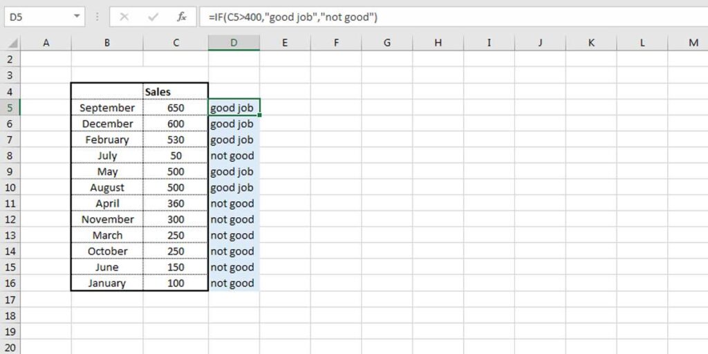
You may need to make a report based on a specific condition. Therefore, IF formulas can help you reach the values you want without having to search them manually. You only need to write a small piece of the formula that contains the statement you have and return it with a comment.

 In the example above, we want to write “Good Job” in front of the sales that are higher than 400k and for the sales lower than this amount we want to write “Not Good.” The formula is as simple as follows: 

IFS function is the same as IF but it’s used instead of IF because it can include more than two conditions, so you don’t need to write multiple if functions to see the result. To learn more about the IFS function, check out the “What is the IFs function” blog.  

Conditional Formatting

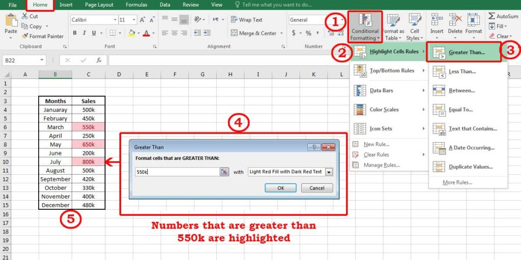
A quick way to analyze data in Excel is by using conditional formatting. This method gives you a quick visual report by formatting the cells that meet specific conditions. The best part is that you can define the formatting, which makes working with them more pleasing. 

1. Select the data you want to analyze.
2. Go to the Home tab.
3. Click on the Conditional Formatting from the Style section.

You can select any of the rules that suit your needs and also choose a format. The cells that meet the condition will change to the formatting you selected. It’s so easy, even if you have a large dataset.  

Charts

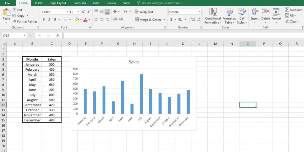
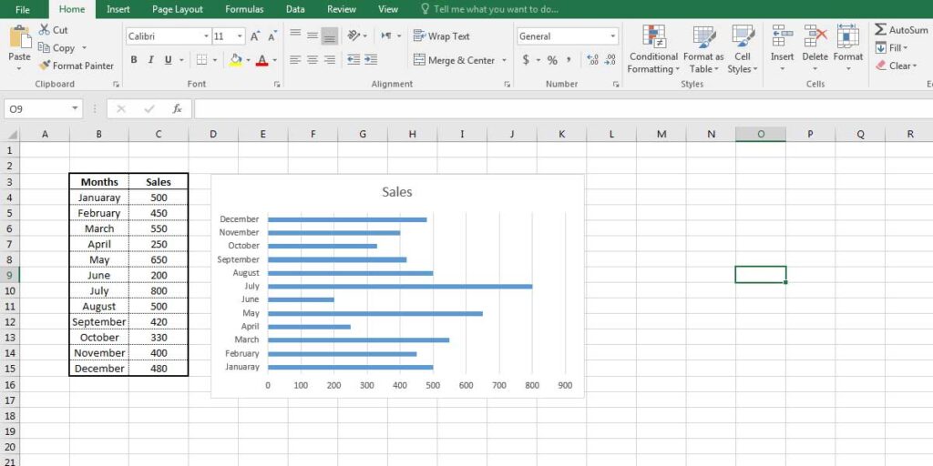
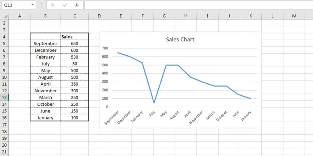
Creating charts is another easy method to visualize data and reports graphically. This is the best option if you want to see the meanings behind numbers and compare them visually. Charts have different appearance and use. For example, if you want to compare the monthly sales you can use Clustered Column or Cluster Bar charts which can show the data in two different colours alongside each other so you can easily find out when you had better sales.

Pie Charts can be used in instances where you want to compare the proportion or quantities to each other and to a whole. For instance, you have a table of your products and you want to know which one sold more. Here, the Pie Chart gets divided into different sections; each part belongs to one product. So, larger sections show more sales.

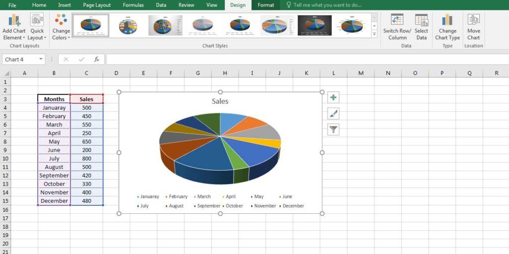
Charts are very useful and easy to apply. You only need to follow these steps: 

1. Select your data

2. Go to the Insert tab.

3. Choose a suitable chart based on your data set.

VLOOKUP

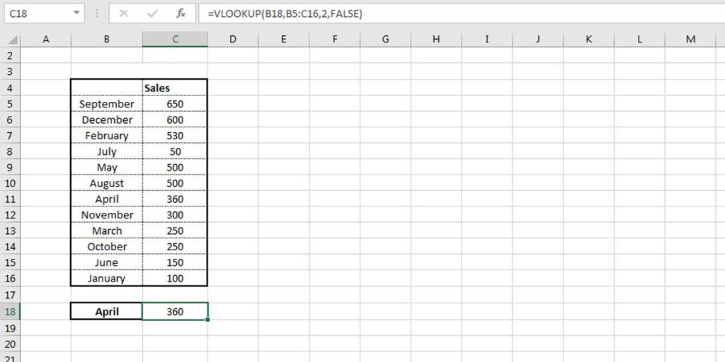
As one of the most useful functions in Excel, VLOOKUP will be your best friend in making reports and data analysis on Excel. Having used this function, you can easily write a formula that calls the value of one cell based on the value of the cell next to it. For example, if you want to know the price of a product, you write its name and call the price from the cell next to it. That’s why it is called Vertical Lookup because it searches vertically. Let’s see how the formula is written:

VLOOKUP([value], [range], [column number], [false or true])

As the formula indicates:

•  [value]: you select from which cell the formula should be read 
• [range]: choose a range from which the formula should check for the value, make sure you select the whole data so the function can read different cells.
• [column number]: Now it’s time to tell VLOOKUP which column it should check, so write it in digit form. 
• TRUE or FALSE is used to inform the function if it is allowed to return an Approximate Match or you only want to have the Exact Match of what you have written. 

Check the following example:

HLOOKUP 

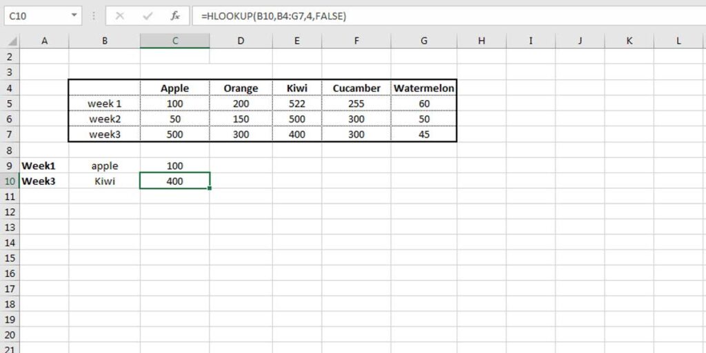
VLOOKUP and HLOOKUP do the same functions. Their difference is that unlike VLOOKUP, which reads the formula vertically, HLOOKUP does the same horizontally. It is used when you have a table whose contents are in the rows below each other. Thus, if you want to search for a value, you need to check the table horizontally. The formula is also the same:

HLOOKUP([value], [range], [row number], [false or true])

LEN

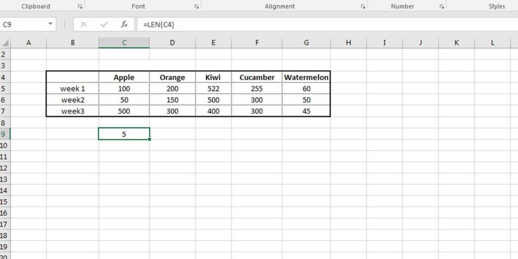
The Excel LEN function is a simple and easy way to count the characters on a cell, regardless of data being in  text or number. The LEN function can read the cell value and return the number of characters. You should note that the space between the characters is also counted, but the formatting does not count. You can call a specific cell to count its characters or directly write the string you want to count. Here is the example:

=LEN(“apple”)

Or 

=LEN(B2) 

See the result below: 

CONCATENATE

The CONCATENATE function is one of the easy functions which brings together the values of different cells in one cell. It is helpful when you need to gather the information, such as the address, product SKU or any other information that is normally entered in different cells. The function is simple and useful, just write the formula as below:

=CONCATENATE (select first cell, select second cell, …) 

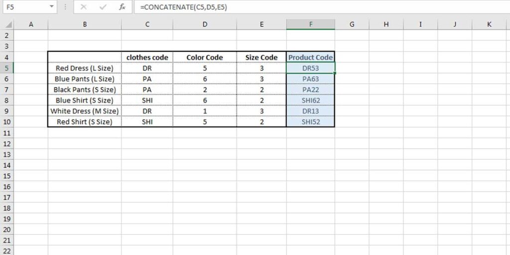
Make sure to add SPACE between each cell if it’s necessary. 

SUMIF

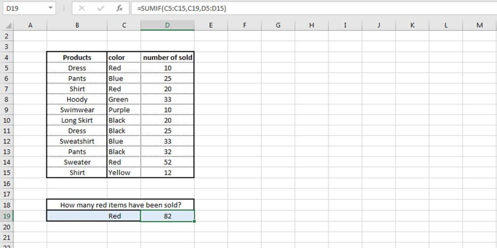
SUMIF is the combination of SUM and IF functions. It means that it will calculate the value of cells in case it meets a single condition, which can be defined by logical operators (> ,< ,<> ,=), or a string – written inside ” “- or a value in a cell. SUMIF function is written as follow:

=SUMIF (range, criteria, [sum_range])

1. Select the  range in which you want the criteria to be true

2. Mention the condition you want the selected cells to have

3. Dedicated to the calculation

 Check the following example:

Solver 

The Solver is not actually a predefined function in Excel, it’s an add-on that you can add whenever you need. Therefore, you should first add it to your Excel and then follow its instructions. But, what does it do, and how can it help you with the analysis?

Assume you want to set a goal for your work, but this goal depends on a complicated condition. Let’s say you want to buy new equipment for your work, and pay its price in 12 months. You consider having 50 customers per month but don’t know how much they should pay for your service. In this case, the Solver can solve your problem!

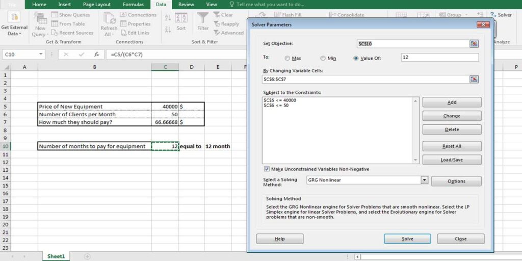
You may think it’s easy to calculate, but you are not sure about the number of customers, so it is variable. Therefore, you should write a formula to consider this change. 

Bottom Line 

Excel has made it easy to analyze and create complicated reports in your business. The functions can help you do your task effortlessly and fast. You don’t need to spend all day calculating different values, instead, you can write a formula and see the result in the blink of an eye.