Mastering Excel Financial Formulas: A Comprehensive Guide for Beginners and Beyond

As a financial analyst or a business accountant, Excel will be your best friend throughout your career. It has numerous functions for formulating assumptions, analyzing risk, and preparing financial strategies. Considering the large number of Excel financial formulas for different data types, it is fairly easy to use Excel for finance. Whether you are an accountant, investor, or corporation, you can perform different technical calculations and prepare the most complex reports and analyses using Excel. Follow this blog post to the bottom line to learn the most applicable Excel financial formulas examples.

I. Basic Excel Financial Formulas

Let’s start our journey with basic Excel formulas as the groundwork for more complex analysis.

A. Sum function

The SUM function allows you to add up a series of numbers in a range of cells. You can use this function for various purposes such as calculating total sales, expenses, or profits.

Syntax: =Sum(number1, [number2], …)

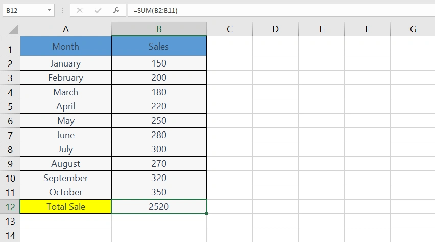
Example: in this table, we have the monthly sales of a product in cells B2 to B11. This formula will give you the total sales for 10 months:

=SUM(B2:B11)

Empower your business with our Excel Programming and VBA Macro Development Services, tailored to automate tasks and unlock the full potential of your data management capabilities.

B. Average function

The AVERAGE function is used to find the mean of a group of numbers. In financial analysis, this function helps you calculate the average sales, expenses, or profits.

Syntax: = AVERAGE(number1, [number2], …)

Example: in the previous data table, we can calculate the average sale in ten months, using this formula:

=AVERAGE(B2:B11)

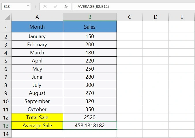
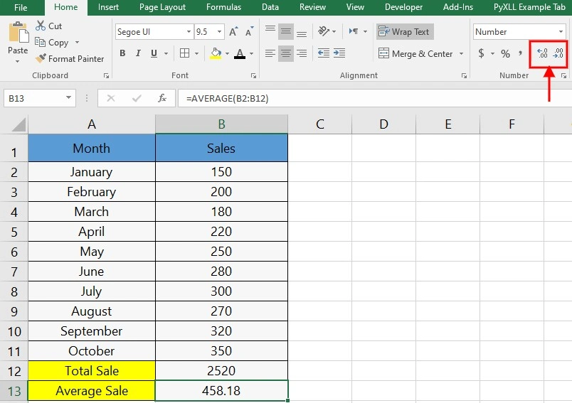
you can increase or decrease decimals in the average value using these icons in the number section: 

C. Count function

The COUNT function is used for counting the number of cells that contain numbers. You can use this function to count items, like the number of transactions, invoices, or entries within a specific range.

Syntax: = COUNT(value1, [value2], …)

Example: Let’s say you run an online shop and want to figure out the number of days you had transactions within a particular month. You can use this formula to do so:

=COUNT(B2:B31)

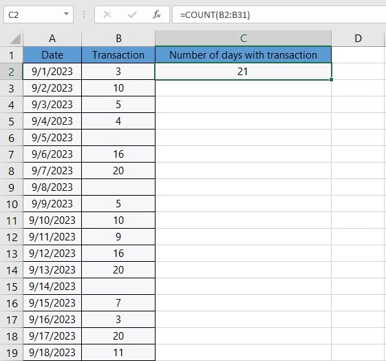
B2:B31 is the range where you have dates of September 2023.

D. IF function

The IF function is a logical function used to make decisions based on specific criteria. You can use this function in cases when the outcome depends on whether certain conditions are met.

Syntax: =IF(logical_test, [value_if_true], [value_if_false])

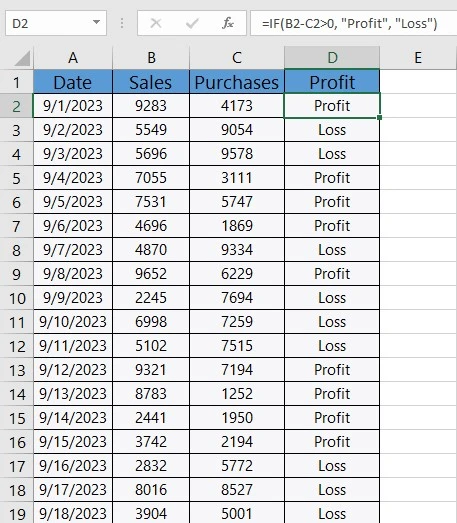
Example: Imagine you have a table reflecting the purchase and sale data within a month.  

=IF(B2-C2>0, “Profit”, “Loss”)

This formula checks if the value of B2-C2 is greater than 0. As you can see in the table, B2 contains the sales data for the first day, and C2 contains its purchase data. If B2-C2>0 is true, it returns “Profit”; otherwise, it returns “Loss”. Drag the fill handle down through the column, and then you can assess whether a particular day’s financial performance was profitable.

Enhance your business efficiency with our specialized Macro Development Services, tailored to automate and streamline your operations for maximum productivity

II. Financial Analysis Formulas

Now let’s move to more advanced parts and cover Excel financial formulas. These formulas such as NPV and IRR in Excel help in evaluating investments, understanding the value of money over time, and assessing the performance of financial ventures.

Transform your financial analysis with our comprehensive Excel Financial Modeling Services, providing accurate and insightful models to drive informed decision-making.

A. Net Present Value (NPV)

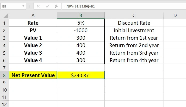
As an investor, it’s critical for you to have a preview of the current value of a future payment stream, known as Net Present Value (NPV). A positive NPV shows that the project or investment will have a positive result. NPV as one of Excel financial formulas can easily calculate this amount. This function actually calculates the net present value of an investment project’s future cash flows using a discount rate.

Syntax: = NPV (Rate, Value 1, [Value 2], [Value 3]…)

Rate: Discount rate for a period

Value 1, [Value 2], [Value 3]…: Positive or negative cash flows, which are considered as payment if negative and inflows if positive.

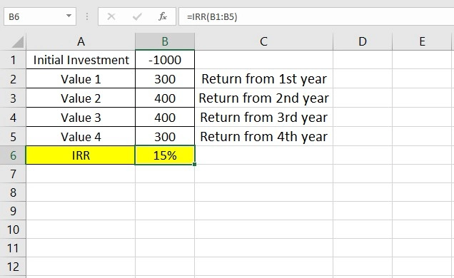
B. Internal Rate of Return (IRR)

IRR, or Internal Rate of Return, is a common variable in financial analysis, used for estimating the profitability of potential investments. It is the discount rate that makes the NPV of a particular project equal to zero. Measuring the IRR index is beneficial for finding the financial justifiability of a project or comparing the investment profitability. It can also help companies decide whether or not to proceed with a project. Among Excel financial formulas, IRR returns a percentage, which shows how profitable a project will be. The result can be positive, which shows it is profitable, and negative to indicate the investment is not a good idea.

Syntax: = IRR (Values, [Guess])

Values: can be an array of values that shows cash flows (it can be negative or positive)

Guess: your assumption about IRR (optional) 

C. Return on Investment (ROI)

Return on Investment (ROI) is a metric, used to evaluate the efficiency or profitability of an investment or compare them in several investments. ROI measures the amount of return on a specific investment, relative to the investment’s cost.

There is no specific ROI function among Excel financial formulas for calculating Return on Investment. Instead, you can calculate ROI with a formula that you input manually.

The basic formula for ROI is:

=((Final Value – Initial Investment) / Initial Investment) * 100

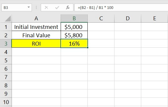
This means your investment yielded a 16% return over the period it was held.

II. Loan and Amortization Formulas

Among Excel financial formulas, there is a group of formulas used in calculating loan payments and understanding amortization schedules. These formulas are indispensable for financial professionals, loan officers, and anyone dealing with credit management or mortgage planning.

A. Loan Payment Calculation

Imagine you have to repay a $1000 loan in 3 years with a constant interest rate of 10%. The loan payment calculation considers the loan’s interest rate, the total number of payments (loan term), and the principal amount borrowed. You can use one of the advanced Excel formulas for this calculation.

PMT function helps you calculate the yearly amount of money you should pay with a certain interest rate. Remember, in PMT, everything is constant, from the interest rate to the final payment.

Syntax: = PMT(Rate, Nper, PV, [FV], [Type])

• Rate: the interest rate of a loan
• Nper: Number of periods you need to make the payment (e.g. 3 years)
• PV: Present Value, the loan you have withdrawn
• FV: Future Value, which is an optional argument, you can leave it empty so it is considered as “0”.
• Type: If you enter 0 in this field, the payment will be made at the end of each period. If you enter 1, the payment will be made at the beginning of each period. (Optional)

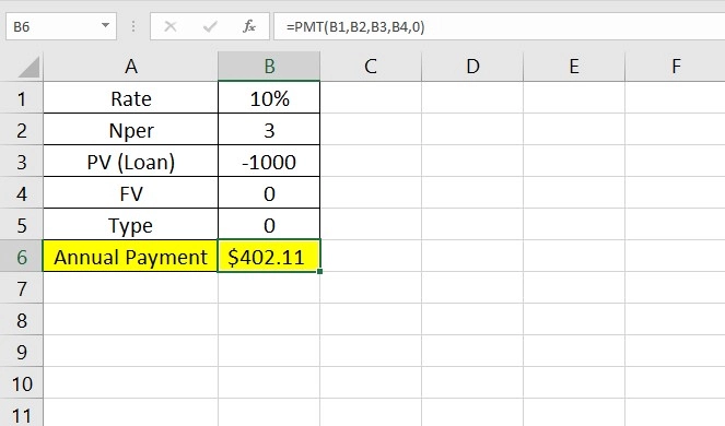
As you can see, if you have to pay back a $1000 loan in 3 years, you need to pay $402.11 annually.

 

 

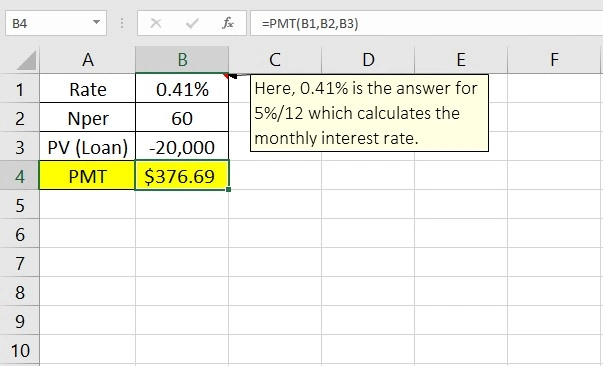
B. Amortization Schedule

Amortization in finance is the process of spreading out a loan into a series of fixed payments over time. The payments account for both principal and interest. An amortization schedule shows the amount going toward the interest and the amount going toward the principal in each payment, along with the remaining balance after each payment. Initially, a larger portion of each payment is devoted to interest; later in the schedule, more of each payment goes toward the principal.

Enhance your business efficiency with our specialized Macro Development Services, tailored to automate and streamline your operations for maximum productivity

Formula for Monthly Payment: =PMT(Rate, Nper, PV)

This formula, as explained above, calculates the fixed monthly payment required to pay off a loan. Imagine you’re taking out a car loan for $20,000. The annual interest rate is 5%, and you plan to pay off the loan over 5 years (60 months).

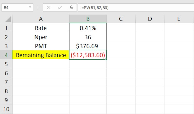
Formula for Remaining Balance: =PV(Rate, Nper, PMT, FV, Type)

This formula calculates the remaining balance of a loan at any given time.

Using the same car loan example above, suppose you want to know the remaining balance after 2 years (24 months) of payments.

Enhance your software capabilities with our customizable Add-In Solutions, seamlessly integrating new features to meet your business needs.

IV. Time Value of Money Formulas

A specific amount of money today has a different value than the same amount in the future due to its potential earning capacity. This fact is based on the time value of money which is a fundamental concept in finance. Excel financial formulas can calculate the time value of money in terms of future and present values, which are critical in investment analysis and financial planning.

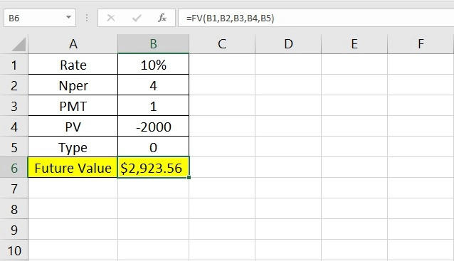
A. Future Value (FV)

Future value is the expected value of the current investment in the future with an assumed growth rate. Knowing the concept of this metric, you can easily write the formula in Excel using the FV function.

Syntax: =FV (Rate, Nper, [Pmt], PV, [Type])

Consider you invested 2000$ in 2020; the payment has been made annually with an interest rate of 10%. The Future Value of this investment in 2024 can be calculated as follows:

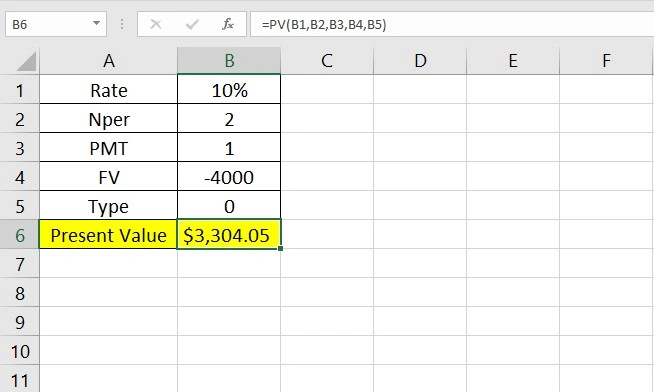
B. Present Value (PV)

Calculating the present value is as effortless as finding the future value (FV). The method and the syntax are all the same, and only the function changes to PV.

Syntax: = PV (Rate, Nper, [Pmt], FV, [Type])

Assume that the future value of an investment is 4000$ in 2026. With a 10% interest rate that has been made yearly for 2 years, we want to know the PV of this amount now (in 2024).

 

 

RATE

V. Advanced Financial Formulas

Advanced Excel financial formulas extend the capabilities of the basic NPV and IRR calculations by allowing for more flexibility in terms of cash flow timing. This is extremely vital in real-world financial analysis since cash flows do not necessarily occur at regular intervals.

Gain expert guidance and maximize your efficiency with our Microsoft Excel Consulting Services, tailored to meet your specific business needs and challenges.

A. XNPV and XIRR

XNPV (Extended Net Present Value) and XIRR (Extended Internal Rate of Return) are advanced versions of the NPV and IRR functions, respectively. These Excel financial formulas are used to calculate the present value and internal rate of return for a series of cash flows that occur at irregular intervals. Thus, they are more practical for real-world scenarios where payments or income do not always follow a standard periodic schedule.

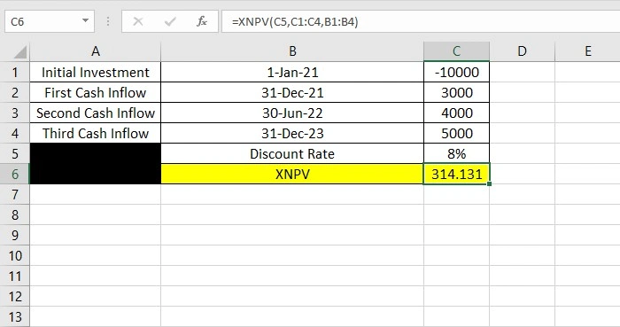
XNPV Syntax: =XNPV(rate, values, dates)

This formula calculates the net present value for a schedule of cash flows that are not necessarily periodic.

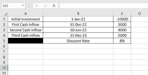
Imagine you are evaluating an investment that involves irregular cash flows. You invest $10,000 initially and then receive cash inflows of $3,000, $4,000, and $5,000 at irregular intervals over the next three years. The dates and cash flows of the investment are as follows:

Using the XNPV function, you can calculate the net present value.

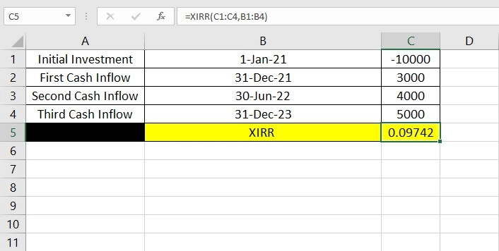
XIRR Syntax : =XIRR(values, dates, [guess])

This formula calculates the internal rate of return for a series of cash flows occurring at irregular periods.

Let’s use the same investment example as above to calculate the XIRR. You want to find out the internal rate of return for this series of irregular cash flows.

VI. Tips and Best Practices

While Excel financial formulas are powerful tools for analysis and decision-making, their effectiveness depends on how they are used. Here are some Excel tips and best practices to enhance the efficiency, accuracy, and clarity of your financial analysis.

A. Using Named Ranges for Clarity

Named ranges in Excel are a way of naming cells or ranges of cells to make formulas easier to understand. Instead of using cell addresses, which can be hard to remember and interpret, named ranges allow you to use descriptive names, making Excel financial formulas more readable.

Tip: Use names like “InitialInvestment”, “AnnualCashFlow”, or “LoanTerm” to refer to specific cells or ranges. For example, instead of =PV(B1, B2, B3), use =PV(InterestRate, NumberOfPeriods, Payment).

B. Checking for Errors and Troubleshooting Formulas

As errors can easily occur in complex financial models, regular checks are crucial. Excel provides several tools and features, like formula auditing and error checking, to help identify and fix common mistakes.

Tip: Use Excel’s formula auditing tools like ‘Trace Precedents’ or ‘Trace Dependents’ to see which cells affect or are affected by a formula. Also, pay attention to error values like #DIV/0!, #VALUE!, or #REF!, and use Excel’s error-checking function to identify and correct them.

C. Keeping Formulas Dynamic with Cell References

One of Excel’s strengths is its ability to automatically update calculations when input values change. By using cell references and avoiding hard-coded numbers in your formulas, you can ensure that your financial models remain dynamic and adaptable.

Tip: Instead of inserting a value directly into a formula, refer to a cell where this value is inputted. For instance, use =FV(InterestRate, Years, -Payment, -Principal) instead of =FV(0.05, 10, -100, -1000).

VII. Conclusion

As you realized through this post, Excel financial formulas are powerful tools to help you with financial analysis. We mentioned only a few of these functions, but you can find them all under the Financial category of the Excel Function list. Whether you are a financial expert or only interested in finance, Excel has made it easier for you to perform different calculations within the finance context. You only need to know some financial spreadsheet techniques, and Excel will do the rest for you.

Need help with financial reports and calculations? Reach out to our Excel Consultant experts for a quote on our Excel services.

FAQs