How To Divide In Excel | 3 Simple Ways
Unlike the SUM function that can automatically add cells’ values in Excel, there is no predefined division function in Excel. However, there are also several ways to do this math operation in this program. To read more about how to divide in Excel, follow this post to learn basic to advanced division methods in Excel.
In case you need a refresher on how to perform basic calculations like subtraction, check out our guide on how to subtract in Excel.
How to divide in Excel
Divide in Excel by using the divide symbol
The simplest way to divide in Excel is by using the divide symbol (/). You can divide numbers into one cell or divide the amounts of multiple cells. We are going to explain each of them as follow:
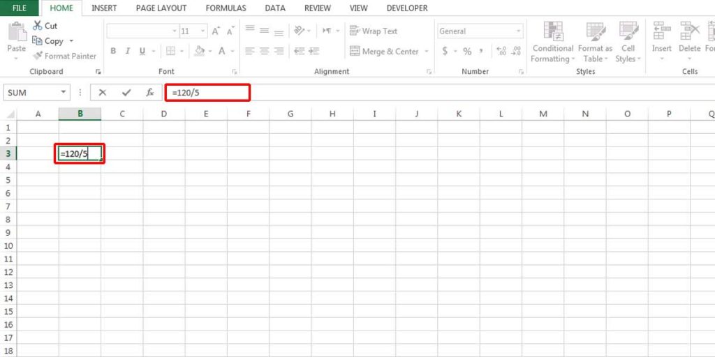
First, to divide two amounts in one cell:
- Select the cell that you want to apply the divide operation to.
- Every formula in Excel should start with “=” so, write this symbol first.
- Write the first number, and without any space, write / and then the second number.
- Press Enter to see the result.
Remember, writing formulas with this method is not always useful. It is more practical to divide the amounts of two different cells. Consequently, if you change the value of each cell, the result will change.
First, write the number in different cells.
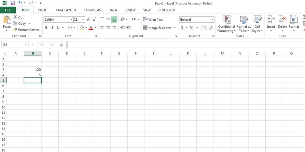
- Select the third cell where you want to display the result. It can be any cell on the sheet. (in our example we chose B5)
- Start the formula by writing an equal sign “=”.
- Select the first cell by clicking on it. (in our example it is B3)
- Write “/” and select the second cell. (in our example is B4)
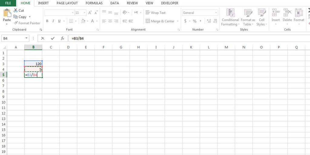
- Press Enter to see the result.
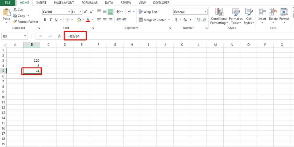
Whenever you modify the value of the cells (in our example B3 and B4), the number in the third cell (here B5) will change. But you can’t write anything in the cells that have formulas. If you double-click on it, you can only see the formula.
Enhance your business efficiency with our specialized Macro Development Services, tailored to automate and streamline your operations for maximum productivity
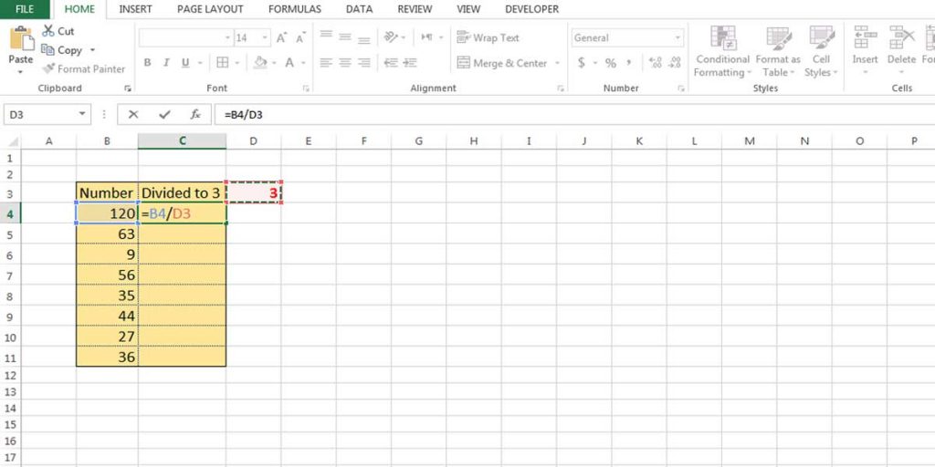
Divide from one cell
Sometimes you may need to divide the value of different cells from the same number. For example, all the cells of one column should be divided into 3.
- Select the cell where you want to see the result. Write an equal symbol “=” and select the first cell.
- Add “/” to the formula and then select the cell that you have written the number. Then press Enter.
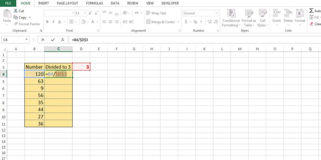
Although it’s possible to write the formula for each cell one by one, it’s easier to fix the cell where you input the number (in this example, D3). So, you can copy the formula for other cells.
- Go to the formula and put the cursor behind the cell name (D3) and press F4. You can see that two dollar signs appear, one before the cell name and the other after that. It shows that this cell (D3) is locked and won’t change by copying.
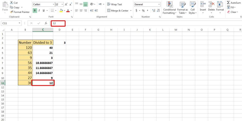
- You can either double-click on the right corner of the cell to copy it to all the other cells which have values or simply drag it down.
What happens if you don’t lock the cell in this formula?
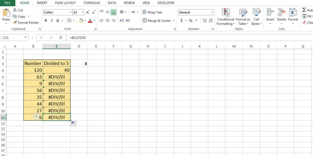
If you don’t lock the cell you want to remain the same for all the formulas, you will face the DIV/O! Error, which displays when the value of the cell you want to divide from equals zero or is not a number at all. Read more on Excel Formula Errors and why they occur.
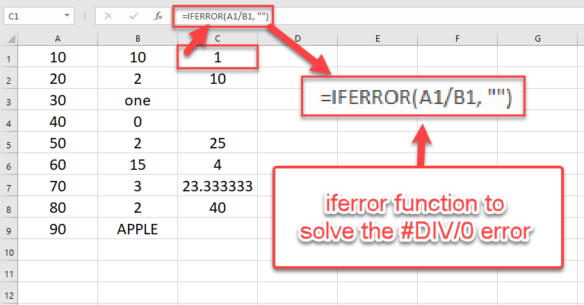
How to Solve #DIV/0!
Since dividing a number by zero is not defined, Excel shows the #DIV/0! Error. A textual or an empty cell will be given a zero value in mathematical calculations in Excel. So, we prefer excel shows the open cell instead of a cell that contains an error.
IFERROR Function
By using the IFERROR function, you can solve the #DIV/0! Error. When you write the formula, you can add this function and define a second parameter to represent it instead of the error. Here are the steps to use this function:
- Select a cell or column (based on the numbers of your dataset.)
- Write the equal sign.
- Write IFERROR()
- As the first argument, write the divide formula (as we mentioned before.)
- As the second argument, write the parameter between “”
For instance, don’t write anything if you want excel to show an empty cell.
=IFERROR(the divide formula, “”)
Enhance your productivity and efficiency with our comprehensive Excel Automation Services, designed to simplify complex tasks and save you valuable time.
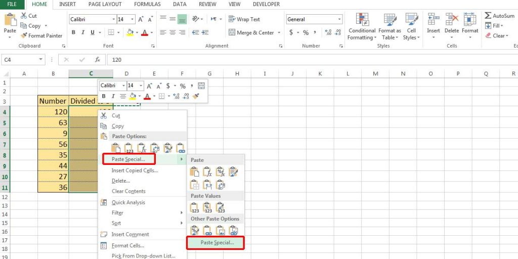
Divide with Paste Special option
As mentioned earlier, if you write a formula in a cell, you’ll see the formula by clicking on it. But, it is also possible to see the value, not the formula. In this case, you should use the Paste Special option. Follow the instruction below:
- In case you want to keep the original values secure, you can make a copy of them to another column. Therefore, select the column and copy it.
- Write the divisor value in another cell. (in our example it’s D3)
- Copy the divisor cell. (The shortcut is Ctrl + C)
- Select the cells you want to divide to this divisor and then right-click and select Paste Special option from the list. (The shortcut is Ctrl + Alt + V)

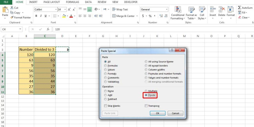
Figure 10- Right-click on the selected cells and choose Paste Special from the list - There are different options in the dialogue box, which is opened. Select Divide, and click OK.
Figure 11- Select Divide from the Paste Special options - The results will appear in the selected cells. Now, if you click on the result cells, you won’t see any formula.
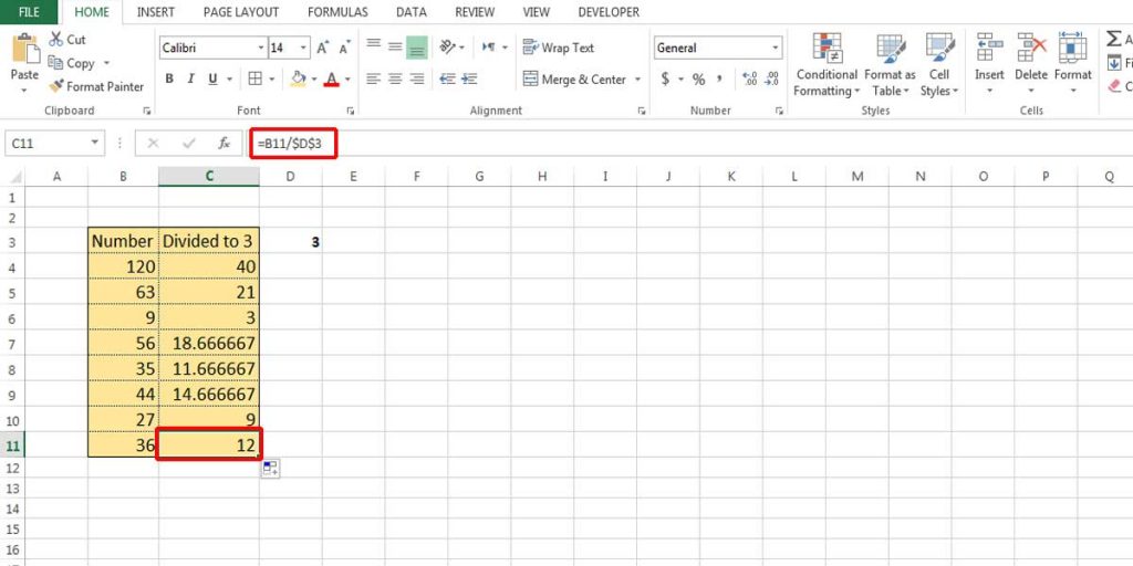
There is one problem with this method of division in Excel. Since you don’t have any formula, if you change the value of the first cells, the result will not change. That makes it a first-time division method, and it’s not dynamic like the division formula in Excel.
Bottom Line
The division is one of the main mathematical operations that are very useful in accounting functions or making different dynamic reports. We explained how to divide in Excel step by step. So, with a little creativity, you can easily use this operation in Excel.
Check out our other blogs, explaining the other three basic arithmetic operations in Excel:
Our experts will be glad to help you, If this article didn’t answer your questions. ASK NOW
We believe this content can enhance our services. Yet, it’s awaiting comprehensive review. Your suggestions for improvement are invaluable. Kindly report any issue or suggestion using the “Report an issue” button below. We value your input.


