How To Multiply In Excel In Office 2010
If you want to use the multiplication function in Excel and you don’t know how to do it, then you’re in the right place.
We are going to go over everything about multiplying in Excel.
Note: When you use multiple operators to write a formula, observe the computational priority of these operators. Consider the term PEMDAS for this purpose.
- Parentheses
- Exponentiation
- Multiply and Division
- Addition and Subtraction
Multiplication in Excel
Actually, doing multiplication in Excel is not that hard, it’s pretty simple, and we’re going to walk you through it.
To multiply your data in Excel, different methods are available.
To write a multiplication formula in Excel, just like any other function, you start with putting a “=” (equal) symbol in the formula bar.
Transform your financial analysis with our comprehensive Excel Financial Modeling Services, providing accurate and insightful models to drive informed decision-making.
Multiplication function in Excel
If you type “=multiplication” in the formula bar in Excel, you’ll see that such a function isn’t available. But it doesn’t mean that you can’t use multiplication in Excel.
The multiply function in Excel is defined as “PRODUCT.”
In the following sections, we’ll see how to use the “PRODUCT” function to multiply numbers, cells, columns, and rows.
Note that using “=PRODUCT” is not the only way to multiply numbers in Excel. And we’ll discuss other techniques as well.
Multiplication formula in Excel
Multiplication formula using (*)
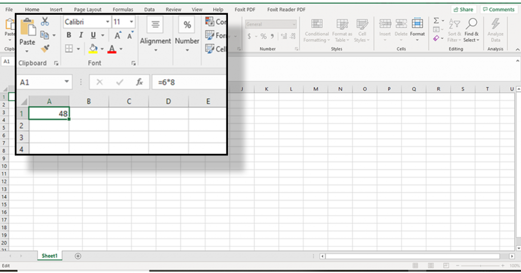
In this formula, the asterisk (*) represents multiplication; for example:
“=6*8”
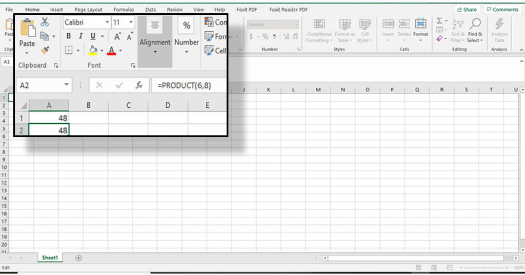
Multiplication formula using PRODUCT function:
In this formula “PRODUCT” represents multiply function; for example:
“=PRODUCT (6;8)”
Boost your productivity by getting a free consultation from Excel experts, and discover tailored solutions to optimize your data management and analysis.
How to multiply cells in Excel?
As we explained before we can use either “PRODUCT” or (*) as the multiplication symbol.
Sometimes we enter numbers in the formula and sometimes we prefer to enter a cell.
Let’s see how it’s done.
Multiplication with (*) and numbers
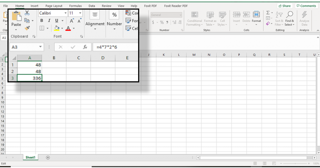
You can use the asterisk (*) to multiply as many numbers as you like:
For example, if you are willing to write a formula that multiplies 4,7,2, and 6; you should type:
“=4*7*2*6”.
The result which is shown in the cell is 336.
Multiplication with (*) and cells
If you want to write a formula that multiplies A1, A4, and B6; you should type:
“=A1*A4*B6”
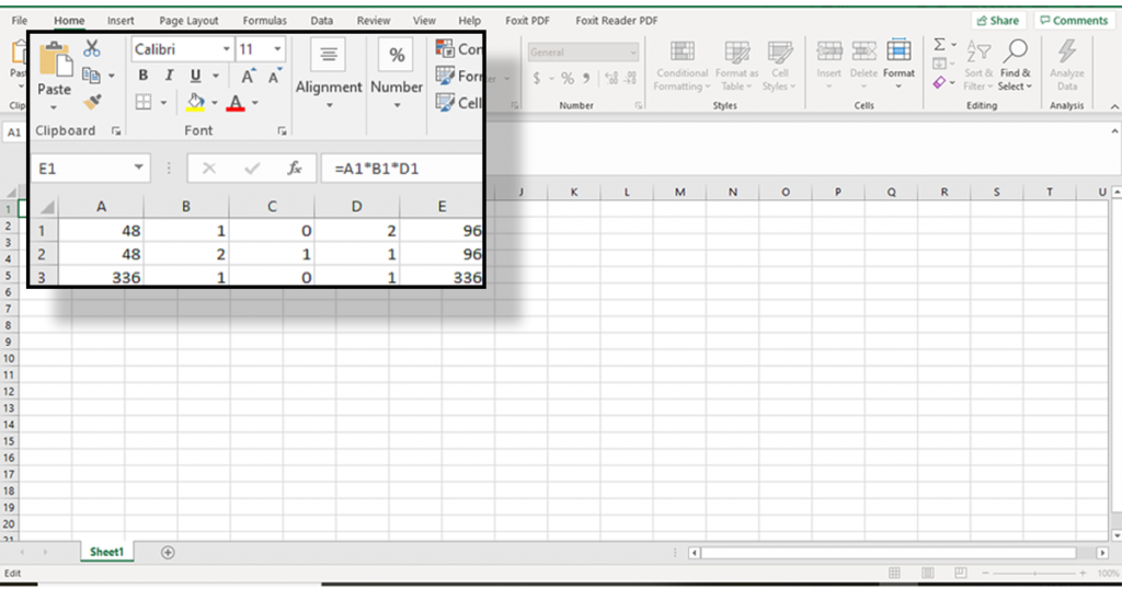
The result will be the multiplication of the values in cells A1, A4 and B6.
To extend this formula, drag the cell down to the selected row.
- You also can click on the selected cells while writing the formula, instead of typing the cell’s name.
- To multiply a cell by a fixed number, just put the fixed number (for example 6) inside the equation:
“=6*A1*A4*B6”
Multiplication by the Paste Special
Doing multiplication without formulas or functions could be done by the Paste Special option in Excel. However, the point is that no dependent cells will be formed since you did not use any formula to perform the multiplication operation in this method. In other words, the multiplication result will not change by changing cells.
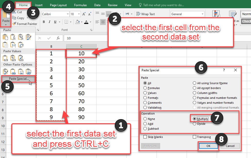
For example, assume we want to multiply two columns, B and C, simply, follow these steps:
- Select your data from the first column.
- Copy these data by CTRL+C shortcut key.
- Select the first cell from the second column.
- Go to the Home tab and click the Paste Special. You can also use the shortcut key by pressing CTRL+ALT+V.
- In the Paste Special dialogue box, go to the Operation, check the Multiply and click OK.
Having done this, the result will appear in column C.
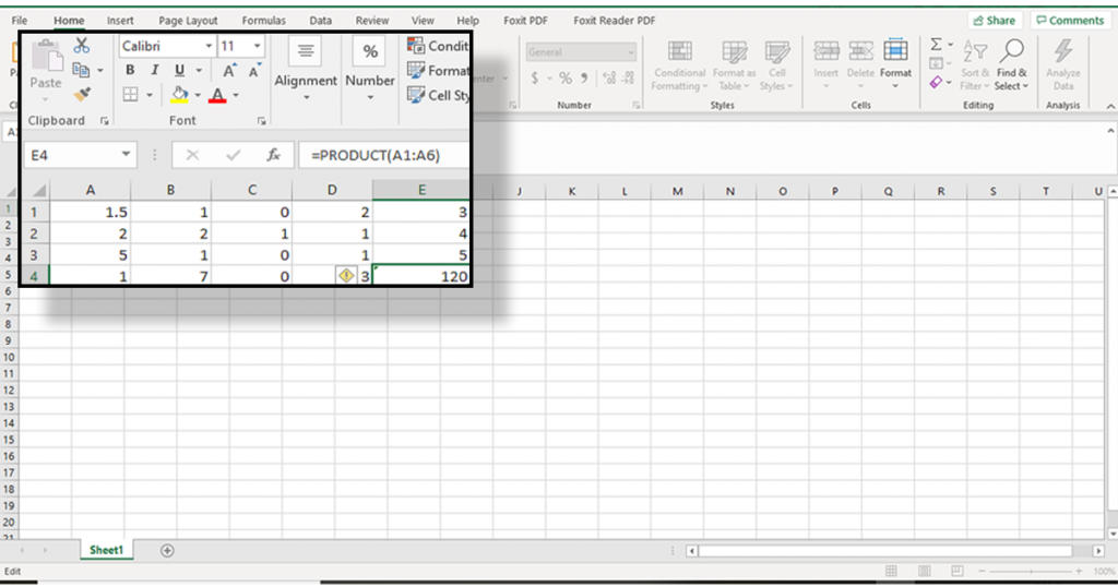
Multiplication with PRODUCT function and numbers
PRODUCT function is actually a shortcut to writing multiplication formulas in Excel.
Let’s consider the previous example again:
If you want to write a formula that multiplies 4,7,2, and 6; You can use PRODUCT function:
“=PRODUCT (4;7;2;6)”
Multiplication with PRODUCT function and cells
To write a formula that multiplies A1, A4, and B6; you should type:
“=PRODUCT(A1*A4*B6)”
- To multiply a range of data (for example A1, A2, A3, ans A4), you can easily type:
“=PRODUCT (A1:A4)”
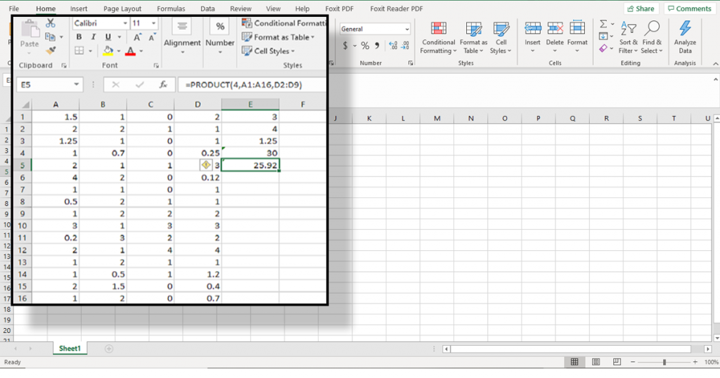
- You can put any combination of, formulas, ranges, cells, and numbers in this formula; for example:
“=PRODUCT (4; A1:A16; D2:D9)”
Enhance your productivity and efficiency with our comprehensive Excel Automation Services, designed to simplify complex tasks and save you valuable time.
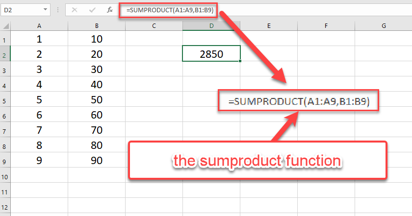
SUMPRODUCT and IMPPRODUCT
The SUMPRODUCT is a function that calculates the summation of product results. For example, assume we have two columns A and B. To use this function, follow these steps:
- Select an empty cell.
- Write the syntax of the function
=SUMPRODUCT(array1, array2, [array3], …)
- Select column A as the first argument and Column B as the second argument.
- Press Enter.
How to Multiply Complex Numbers in Excel
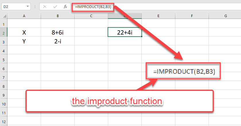
To do engineering calculations in Excel, we often use complex numbers. As you know these type of calculations are different from how we calculate Real numbers, such as multiplying the complex data by the IMPRODUCT function.
For instance, we have two complex numbers:
X=8+6i
Y=2-i
We can multiply these two by the =IMPRODUCT(X, Y) and see the result quickly.
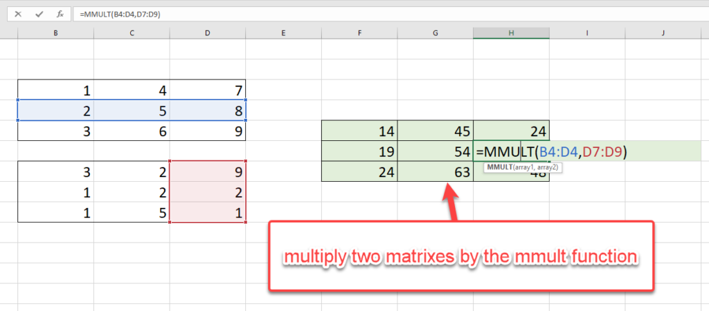
How to multiply Matrices
If you’re already familiar with multiplying two matrices, you know that these calculations are awfully long. Here, Excel does the multiplication in a blink of an eye and shows the result immediately by the MMULT function.
To use this function, please proceed as follows:
- Select an empty cell.
- Write this function or find it in the Math and Trig group of the Formula tab.
The MMULT function syntax is:
=MMULT(array1, array2)
- Select the first matrix as array1 and the second matrix as array2.
- Press CTRL+SHIFT+ENTER to see the result.
Note: The #Value! error means that the matrixes include an empty or textual cell or the first matrix column number is not equal to the second matrix row.
In this blog, we attempted to cover the main techniques and tips concerning multiplication in Excel. Multiplication is also known as Product in Excel. If you know any other interesting technical points please let us know in the comments. Make sure to contact us if you need further information about Excel service and solutions our team of experts provide for your business.
Don’t forget to check out our other blogs, explaining the other three basic arithmetic operations in Excel:
Our experts will be glad to help you, If this article didn’t answer your questions. ASK NOW
We believe this content can enhance our services. Yet, it’s awaiting comprehensive review. Your suggestions for improvement are invaluable. Kindly report any issue or suggestion using the “Report an issue” button below. We value your input.


