How To Merge Cells In Excel

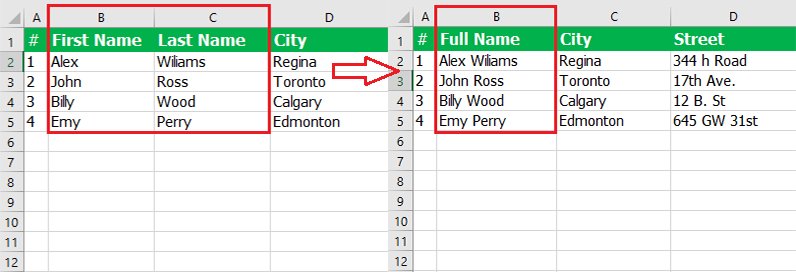
In this article, we’re going to learn how to combine multiple columns in Excel into one column without losing any data. Suppose you have a table in Excel, and you’d like to merge two columns, line by line. For example, let’s think that you want to merge the “First name” and “Last name” columns together to create a “Full Name” column or that you want to merge the columns of “City,” “Street,” and “Postal Code” into a single “Address” column.

Unfortunately, Excel does not offer an internal tool for merging columns.

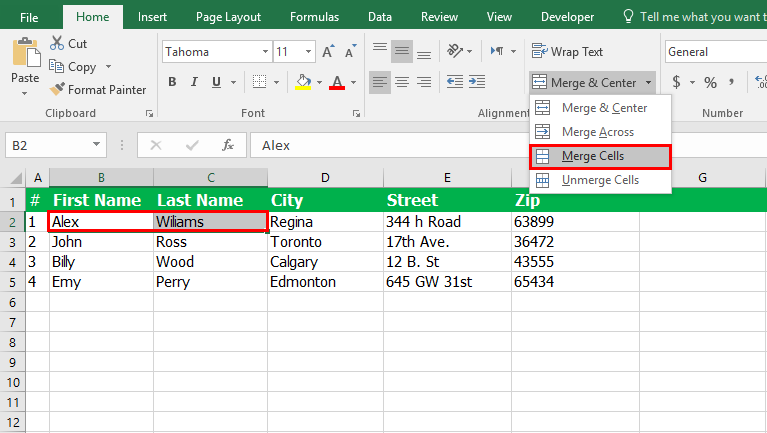
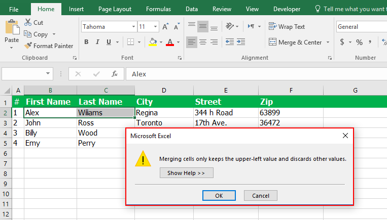
If you use the “Merge” button for combining two adjacent columns, you will likely see the following error: “Merging cells only keeps the upper-left cell value and discards the other values.” (Excel 2013) Or “The selection contains multiple data values. Merging into one cell will keep the upper-left most data only.”(Excel 2007, 2010)

In this article, we’re going to look at two different methods for merging columns in Excel without losing any data or having to use VBA macros.

 

 

Merging Two Columns in Excel Using Formulas

For instance, let’s think that you have a table containing your customer’s personal information and you would like to merge the “First name” and “Last name” columns into a “Full Name” column.

1. Let’s create a new column. Move the mouse cursor to the column area (column D in our example) right-click on it and select “Insert.” Name the new column “Full name.”
2. In cell D2, enter the following formula: =CONCATENATE(B2,” “,C2)

Here, B2 and D2 are the cells for First and Last name, respectively. Please note that there is a single space between the two quotation marks in the formula; This is a separator for the First and Last names in the new column. You could use any other sign as a separator, for example, a comma.

Using a similar method, you can merge data from different cells using any sign as the separator. For example, you can combine data from three different columns (City, Street, Zip) into one cell.

3. Copy the formula into every cell of the “Full Name” column. You can hold the plus sign (+) and pull it down to auto-fill the cells.
4. So far, we’ve combined the names of two columns. But this is still a formula. If you delete the First or Last name, the Full Name data will be corrupted.
5. Now we have to convert the formula into a value so we can remove unnecessary columns. Select the cells in the new column which contain data. You can select the first cell and the Press Ctrl+Shift+Down Arrow. Copy the selected cells. Next right-click on the same column and Press “Paste Special” and then select “Values.”
6. Now you can delete the “First Name” and “Last Name” columns. One way of doing this is choosing the title for column B (while holding down Control) and then selecting column C. Then right-click on the columns and select “Delete.” 

https://youtu.be/dOrvxTdexIQ

We’ve now combined the names from two different columns into one column, although it took some effort and time. 

How to Merge and Center in Excel Using Notepad

This method is quicker compared to the last and doesn’t require formulas. But it’s only useful for combining adjacent columns and using a single separator for all data.

Let’s go through the last example again using this method and learn how to merge cells in Excel:

1. Select the two columns. Click on B1 cell and then press “Ctrl+Shift+Arrow Right” to select C1. Then press “Ctrl+Shift+Arrow Down” to select all the cells in both columns.
2. Copy the data. (Press Ctrl+C).
3. Open Notepad. Start > All Programs > Accessories > Notepad.
4. Paste the copied data into Notepad. (Press Ctrl+V)
5. Copy the “Tab” character to the clipboard. Press the Tab button (Tab ↹) on Notepad and then copy the character.
6. Replace the Tab character with your intended separator Press Ctrl+H to open the “Replace” window. Paste the Tab character into the “Find What” field and type the separator into the “Replace with” field. For example, a comma. Finally, press the “Replace All” button.
7. Press Ctrl+A to select all the text in Notepad. Press Ctrl+C to copy the text.
8. Return to your Excel worksheet. Select cell B1 and paste the copied data into the table.
9. Change the name of the B column (“Full Name” in our example) and then delete the “Last Name” column. 

https://youtu.be/hiH4mJuJ-LU

So in this article, we learned how to combine cells in excel. The 2nd method technically has more steps, but it’s quicker than the first. If you don’t believe me, try it out!