How to Randomize Lists in excel + Shuffle Data

There are several options for sorting data in Excel, such as ascending or descending numbers or sorting them alphabetically. But what if you want to randomize a list or select random numbers from the list? Randomizing data is not so common in Excel. However, it doesn’t mean it is not useful. In this post, we will explain to you how to randomize a list in Excel.

How to randomize a list in Excel with a formula (random sort in excel)

You can make a list and allocate a random number to each cell using different formulas. The most commonly used formula is the RAND function, which generates a random number between 0 and 1. After dedicating a random number to each cell, you can sort the numbers and shuffle the list. Here is how it works:

Randomize Columns with RAND function

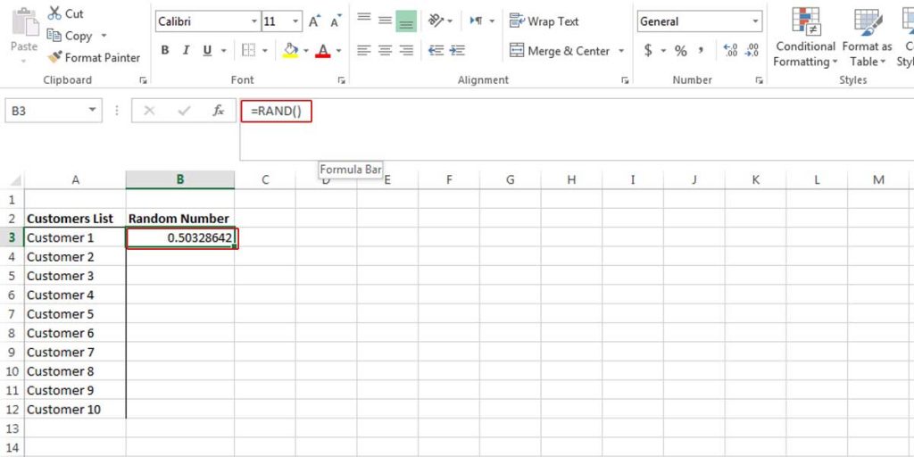
Assume that we have a list of our customers in column A. We want to sort this list randomly. Therefore, we need to have another column to show random numbers. In this example, we named it “Random Numbers.”

1. Click on the first cell in column B and write =RAND() formula and then press Enter; a random number between 0 and 1 appears in the cell.

   

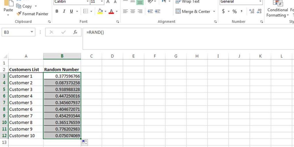
2. Double click on the lower right corner of the first cell so the function will be copied to the rest of the cells.

   

3. Now you can sort the randomized numbers by “sort and filter” from the home tab or from the sort and filter group in the data tab or even round them using the ROUND function.
   

   

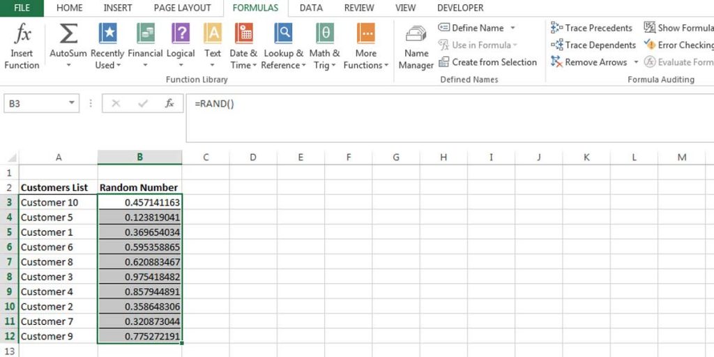
Please note that every time you make a change in cells, the RAND function generates new random numbers. Therefore, by sorting the numbers, you may see new random numbers too. If you don’t want the numbers to change, first, copy the value of the cells in another column, then sort them.

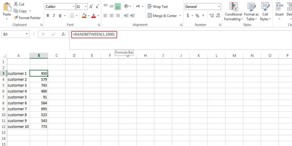
Randomize Columns with RANDBETWEEN function

RANDBETWEEN is another function that can randomize numbers in Excel. In this function, the numbers are randomized between two given numbers. For instance, you want to generate random numbers between 1 to 10. Thus, you write RANDBETWEEN(1,10).

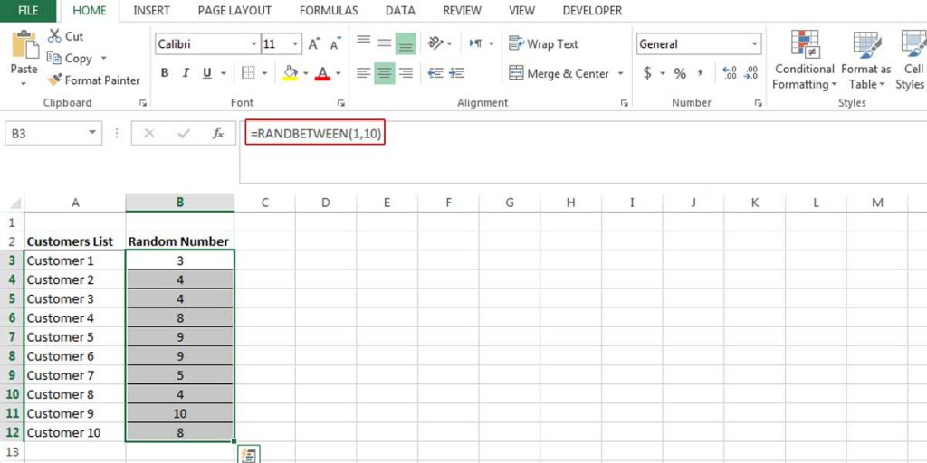
However, as you can see, the problem with RANDBETWEEN is that it may randomize a number twice or even more. This part of randomizing is out of our control; if you want to have a more accurate result, the RAND function will give you more numbers.

If you widen the range between the numbers, for example, randomizing numbers between 1 to 1000, the chance of having a number twice will be less. Therefore, this method will be more useful to have a more unique random number.

To receive expert Excel consulting services, explore our professional services and book a free meeting now!

How to Shuffle Columns and Rows in Excel  (Randomizing Multiple Columns and Rows in Excel) 

If you want to shuffle the data in multiple columns or rows, you can follow these steps. 

1. To shuffle columns, add a column to the left or right side of the table. 
2. To shuffle rows, add a row to the top of the table. 
3. Write the RAND formula in the cells of the added column and row. 
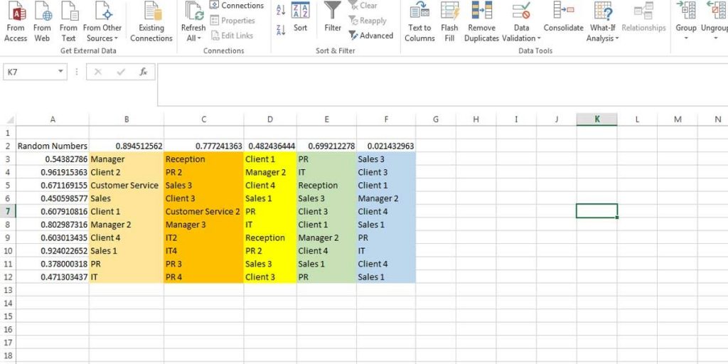
4. Now you have a set of random numbers on top and left sides of the table. Like the sample below.

   

   To make it clear what happens when we shuffle columns and rows at the same time, we have colorized the columns and dedicated data to each of them. Now when it shuffles, we can easily find out what has happened.

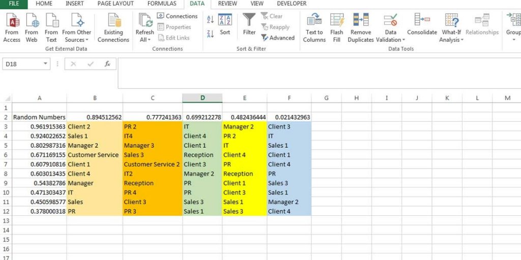
5. Whether you randomly sort the data of rows or columns first, just sort them as you prefer. In our example, we have sorted both columns and rows from largest to smallest.
6. To sort the rows, go to Data> Sort, a window will open, then click on Option and select Sort Left to Right. Then follow the image below.

   

    See the result in the following sample. 

   

It may seem that shuffling the data in columns and rows will shuffle the whole table. The problem here is that the data in this table is shuffled into groups. That means it doesn’t spread the data inside the table; it just sorts the data in column groups. To shuffle more randomly, you need to write a VBA code to work on the whole table.

If you are familiar with writing VBA code for Excel, add the codes below to a module in your worksheet. This code can help you to shuffle columns and rows in Excel more reasonably:

Option Explicit
 
Public Sub ShuffleGrid()
  Dim rngSelected As Range
  Set rngSelected = selection
 
  Dim horizontalLength As Long
  Dim verticalLength As Long
 
  horizontalLength = rngSelected.Columns.Count
  verticalLength = rngSelected.Rows.Count
 
  Dim i As Long
  Dim j As Long
 
  For i = verticalLength To 1 Step -1
    For j = horizontalLength To 1 Step -1
      Dim rndRow As Long
      Dim rndColumn As Long
      rndRow = Application.WorksheetFunction.RoundDown(verticalLength * Rnd + 1, 0)
      rndColumn = Application.WorksheetFunction.RoundDown(horizontalLength * Rnd + 1, 0)
 
      Dim temp As String
      Dim tempColor As Long
      Dim tempFontColor As Long
 
      temp = rngSelected.Cells(i, j).Formula
      tempColor = rngSelected.Cells(i, j).Interior.Color
      tempFontColor = rngSelected.Cells(i, j).Font.Color
 
      rngSelected.Cells(i, j).Formula = rngSelected.Cells(rndRow, rndColumn).Formula
      rngSelected.Cells(i, j).Interior.Color = rngSelected.Cells(rndRow, rndColumn).Interior.Color
      rngSelected.Cells(i, j).Font.Color = rngSelected.Cells(rndRow, rndColumn).Font.Color
 
      rngSelected.Cells(rndRow, rndColumn).Formula = temp
      rngSelected.Cells(rndRow, rndColumn).Interior.Color = tempColor
      rngSelected.Cells(rndRow, rndColumn).Font.Color = tempFontColor
    Next j
  Next i
 
End Sub

Bottom Line 

Randomly sorting lists is so easy on Excel; you first need to add a column or row to add random numbers using the RAND function, and then you can sort those numbers and your list will be shuffled accordingly.