How To Make A Drop-Down List In Excel

Making a drop-down list in Excel lets you regularize your data and avoids making mistakes. You can add options such as YES or NO, FEMALE or MALE, or any other option to a cell too. Also, you are able to limit the value of other cells according to a cell containing a drop-down list. For example, when we select the Canada state, the cities of Toronto, Vancouver, and Montreal are displayed in another cell.

In this tutorial, we will learn about how to add a drop-down list in Excel. Also, we talk about:

• Making lists of names
• Creating a table
• Naming a range
• Adding a dependent list by indirect formula
• Add a third dependent list

Add a Drop Down List 

If you already have a list and only need to create a drop-down list, follow these steps:

1. Create a table.
2. Select the cell you want to enter the drop-down list.
3. Go to the Data tab,
4. Click on the Data Validation from the Data Tools section.
5. Go to the Setting tab from the Data Validation dialogue box.
6. Open the Allow menu, and pick the List.
7. In the Source box, enter the listed range you already have.
8. Press OK.

But if you need to make a list, the following tutorial will guide you through it. Also, we’re going to learn how to make a Professional drop-down list:

Making lists of names

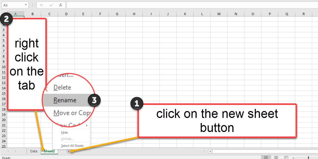
First, you need a workbook containing two worksheets. We named the worksheets “Data” and “Lists.” So open Excel, on the bottom of the worksheet press on  icon, and make a new sheet. By right-clicking on the Sheet1 and selecting Rename (or double click on the tab), you can change the name of sheet1 to Data (for this example), then press the Enter key on your keyboard.

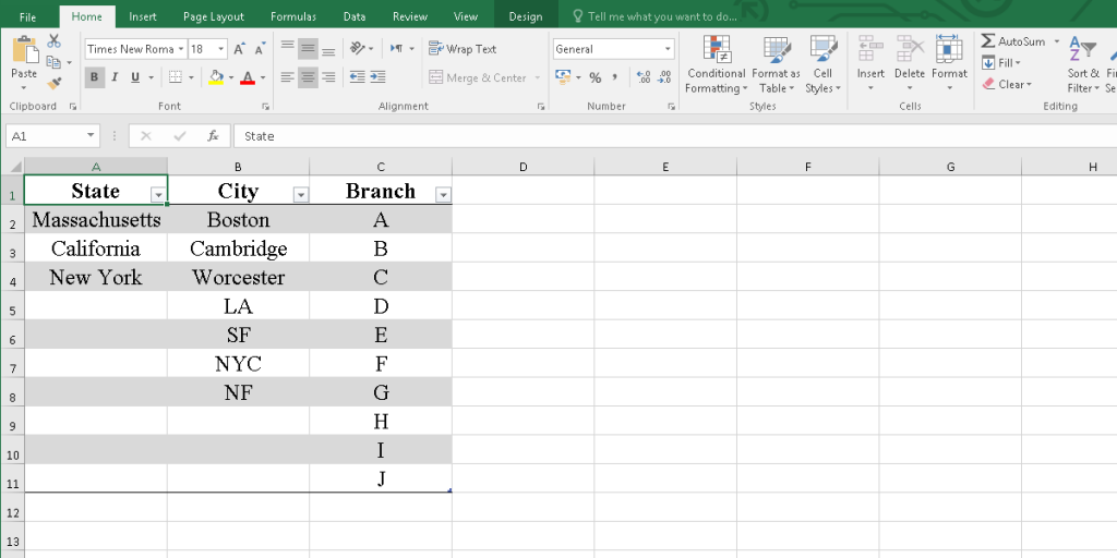
In the Data sheet, we’ll enter lists of names. These lists provide the items needed for affiliate drop down lists. The lists are:

1. State: Massachusetts, California, and New York.
2. City: Boston, Cambridge, Worcester, LA, SF, NY, NF.
3. Branch: A, B, C, D, E, F, G, H, I, and J. 

Creating a table

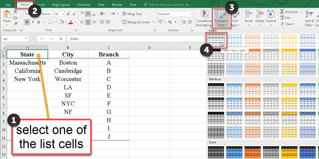
Follow the steps below to create a table with a name for your list. This will make your list dynamic, so new items that are added will be automatically added to your drop down list.

1. Select one of your list cells.
2. Go to the Home tab.
3. From the Style section, click on the Format as Table.
4. Choose one of the styles from the menu.
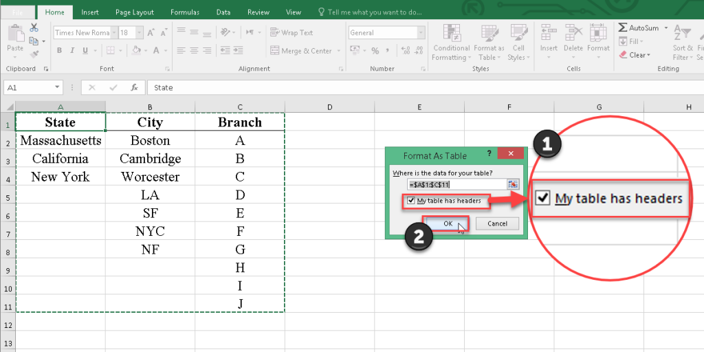
5. Check the My Table Has Headers checkbox.
6. Press OK.

Why should you put your information on the table?

Once your data is in a table, when adding or deleting items in the list,

each slide is automatically updated based on that table.

You don’t have to do anything else.

Naming a range

The next step is naming the ranges of data. So select the state items, and enter the range name on the Name Box next to the formula bar.

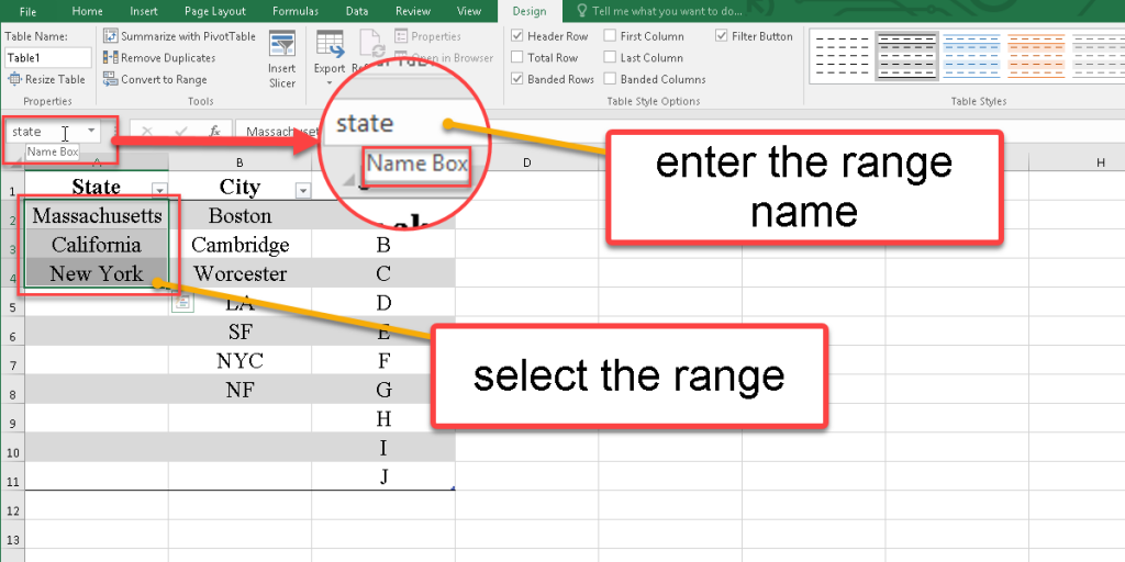
Also, here, we name the “City” range and the “Branch” range.

Create a Drop Down Menu

Based on the previous steps, go to the Lists sheet and follow the steps below to add your drop down list:

1. Enter the titles of your drop down list. In this example, we have three titles; State, City, and Branch.
2. Create a table for each title.
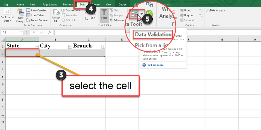
3. Now we select the A2 cell to make a drop down list for the State header.
4. Go to the Data tab from the ribbon.
5. From the Data Tools section, select the Data Validation .

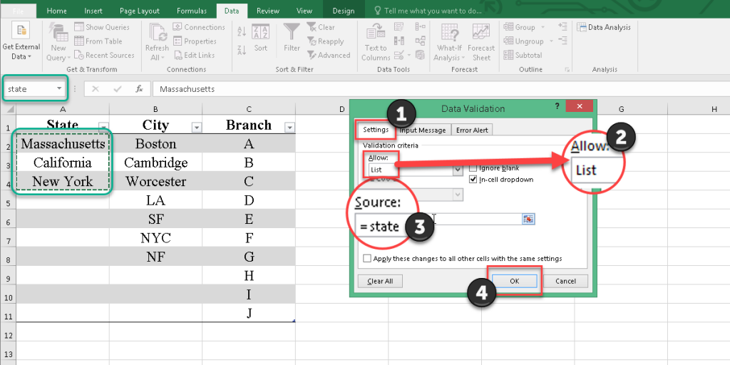
6. Go to the Setting tab from the Data Validation dialogue box.
7. Open the Allow menu and pick the List.
8. In the Source box enter =(the range name that you picked before; here we enter the state which includes Canada, California, and New York)
9. Press OK.

Add a dependent list by the indirect formula

According to the example, we need to display the cities based on the state. So, we create a dependent drop down list in the city column by the Indirect formula. 

Follow the steps in the last section to create a drop down menu but in the Source box (step 8) enter =indirect(the basis cell)

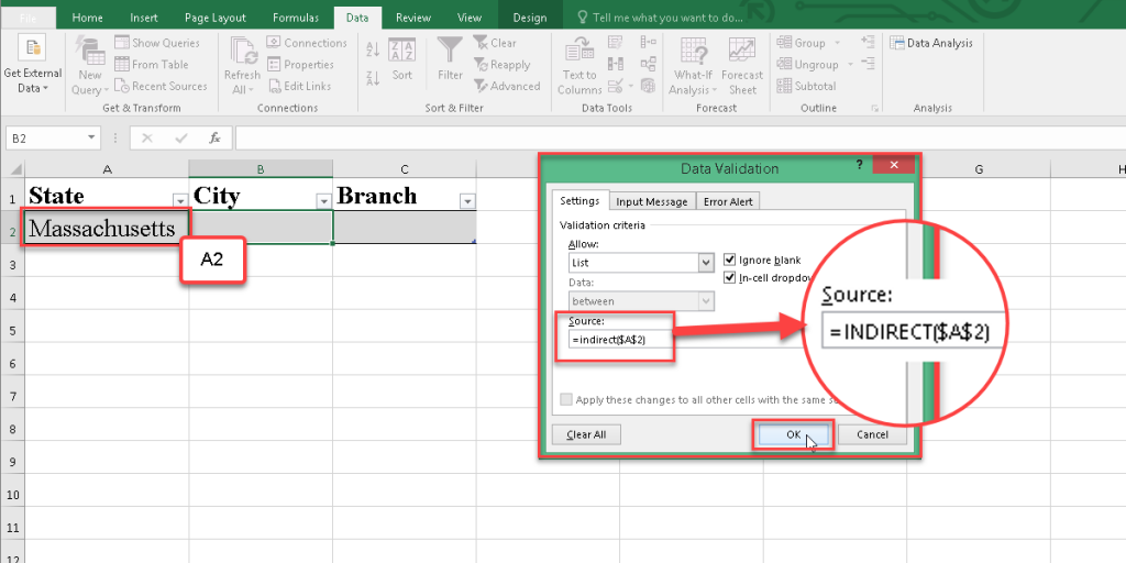
Note: make sure you pick a correct name for each range. Pay attention to this example ranges names in the Data sheet:

• B2-B4 (Boston, Cambridge, Worcester): Massachusetts
• B5-B6 (LA, SF): California
• B7-B8 (NYC, NF): New York
• C2-C3 (A, B): Boston
• C4-C5 (C, D): Cambridge
• C6-C7 (E, F): Worcester
• C8 (G): LA
• C9 (H): SF
• C10 (I): NYC
• C11 (J): NF

You can connect with us and ask our experts for your inquiries and get more Excel Support Services.

Reduce costs, accelerate tasks, and improve quality with Excel Automation Services.