Excel Regression Analysis: Decision-Making Insights

Regression analysis is a statistical method used to study the magnitude and structure of a relationship between a single dependent variable and one or more independent variables. 

Understanding the relationships between variables can enable business owners, executives, and scientists to pinpoint areas for improvement. This can be leveraged to drive strategic planning and decision-making.

 

Linear Regression Use Cases

Regression analysis is used in science and business to: 

• Explain unknown phenomena. e.g. Why did sales drop last month?
• To decide what to do. e.g. Should we plan a different promotion or go with this one?
• Predict things about the future. e.g. What will sales look like over the next quarter?

Regression analysis can be performed using statistics programs like SPSS, STATA, or Excel, as well as programming languages like Python and R. In this blog, we use Excel to perform linear regression analysis on a real-world dataset.

 

Linear Regression Applications

One can find many examples of the usefulness of regression analysis in various fields or domains, such as finance, healthcare, retail, etc. Below are some examples.

• Sales Forecasting:  Regression can be used to predict a salesperson’s total yearly sales from independent variables such as age, education, and years of experience. 
• Psychology: Regression can also be used in the field of psychology, for example, to determine individual satisfaction, based on demographic and psychological factors. 
• Price Prediction: Regression analysis can be used to predict the price of a house in an area, based on its size number of bedrooms, and so on. 
• Income Prediction: Regression can help us predict employment income for independent variables such as hours of work, education, occupation, sex, age, years of experience, and so on. 

 

 

Dependent and Independent Variables in Regression

In regression, there are two types of variables: 

Dependent variable: The dependent variable, which is conventionally noted by Y, can be seen as the state, target, or final goal we study and try to predict. 

Independent variables: There are typically one or more independent variables in a regression model. They are also known as explanatory variables and can be seen as the causes of those states. The independent variables are shown conventionally by x.

A regression model relates Y (the dependent variable) to a function of x_i (the independent variables). The key point in the regression is that the dependent value should be continuous and cannot be a discrete value. However, the independent variables can be measured on either a categorical or continuous measurement scale.

 

Mathematics of Linear Regression

The general form of the linear regression model is:

Y = β₀ + β₁x₁ + β₂x₂ + … + β_nx_n + ϵ

Where:

• Y: The dependent variable
• n: The number of independent variables
• x₁, x₂, …, x_n : The independent variables
• β₀: the intercept
• β₁, β₂, …, β_n: The coefficients of the independent variables, representing their respective impacts on the dependent variable.
• ϵ: The error term. In real life, independent variables are never perfect predictors of the dependent variable. Rather the regression model is an estimate based on the available data. So, the error term indicates how certain one can be about the model. The larger the error, the less certain the regression model is.

 

Essential Prerequisites for Linear Regression

To ensure the validity of linear regression models, four key assumptions must be met.

• Linearity:  Linearity means that the data must look like a line when plotted on an x, y coordinate plane, i.e. points on the plot appear to fall along a straight line. If the scatter plot looks like a random cloud or resembles a curve rather than a line, then the assumption is invalidated, meaning that the linear regression model does not fit the data well. In that case, we might need a different or more complicated model for this dataset.

• Normality: This assumes that the residual values or errors are normally distributed. Since this assumption is about residuals, it can not be checked until after the model is built. However once the model is created, a quantile-quantile or QQ plot of the residuals can help. If the points on the plot appear to form a straight diagonal line, then we can assume normality and check this assumption off the list. 
• Independent Observations: Independence states that each observation in the dataset is independent. To check for independence, it is helpful to use contextual information about data collection and the variables to determine if this assumption is valid. If the assumption is met, we would expect a scatter plot of the fitted values versus residuals to resemble a random cloud of data points. If there are any patterns, then we might need to re-examine the data. 
• Homoscedasticity: Homoscedasticity means having the same scatter. Scatter plots come to the rescue once again when checking for homoscedasticity. Returning to the scatter plot of fitted values versus residuals, there should be constant variance along the values of the dependent variable. This assumption is true if no clear pattern can be noticed in a scatter plot. Sometimes homoscedasticity is described as a random cloud of data points.

 

Scenario and Dataset

TiTi is a toy retail company that sells various kinds of toys in the local market. The sales manager needs to make projections about the impact of unit price, advertisement, and promotions on the number of monthly units that the company will be able to sell of a particular toy in the coming month. In the past, she has been making such projections based on her experience. Now she wishes to be a little more data-driven about the whole process. She has collected the sales data for 24 months in an Excel file.

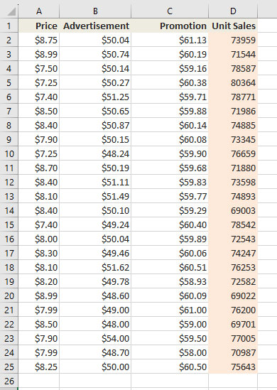
The rest of this article is devoted to conducting linear regression analysis in Excel.  This will help the sales manager deal with the situation more systematically rather than relying on her gut feeling. We will then interpret and assess the credibility of the result. In the end, we will use the model to predict the outcome for an unknown input.

The reader of this blog is supposed to be familiar with the theories of linear regression and have a working knowledge of Microsoft Excel.

 

Setting up Excel for Regression Analysis

To perform regression analysis in Excel, you need to enable the Analysis Toolpak add-in. Keep in mind that these steps are for Excel in version 2021 and may vary slightly in your version of Excel.

1. Click File > More > Options. 
2. In the Excel Options window, select Add-Ins on the left sidebar.
3. In the Manage dropdown box select Excel Add-ins then click Go.
4. In the Add-Ins box, tick off the Analysis Toolpak check box, then click OK. This will add the Data Analysis tools to the Data tab of your Excel ribbon.

• If you do not see Analysis ToolPak listed in the available Add-ins, click Browse to find and select it.
• If you receive a prompt indicating that Analysis ToolPak is not installed on your computer, click Yes to initiate the installation process.
•  

 

Linear Regression in Excel

Carry out these steps to perform linear regression analysis in Excel.

1. Select the Data tab -> Analyze -> Data Analysis. This will open the Data Analysis window.
2. Choose Regression, then click OK.
3. In the Regression dialog box, set the Y-Range, and X-Range to be your independent and dependent variables respectively.
4. Set other variables according to your needs.
   1. Labels box: If there are headers at the top of your X and Y range.
   2. Output options: select where you want the regression output to appear (e.g., a new worksheet).
   3. Residuals: get the difference between the predicted and actual values.
5. Click OK.

 

Interpreting Regression Analysis Output in Excel

The regression output has three components:

• Regression Statistics
• ANOVA
• Regression Coefficients

Regression Statistics

Gives the overall goodness-of-fit measures.

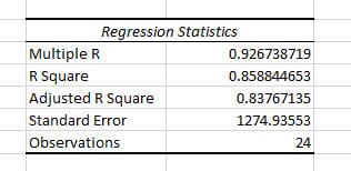
• Multiple R
  • The square root of R-squared
  • Correlation between Y (actual Y) and Y-hat (estimated Y)
• R-squared (R²): 
  • Measures how much of the variability in the dependent variables is explained by the model. It can be a value in the range of [0,1] inclusive. Higher values indicate a better fit of the model.
  • R²= 0.8588 means that 85.88% of the variation of Y (Unit Sales) around  its mean is explained by the regressors (Price, Advertisement, and Promotion)
• Adjusted R Square
  •  Used for cases with more than one x variable.
  •  = R² – (1-R² )*(k-1)/(n-k). k: number of residuals including intercept, n: number of observations
• Standard Error
  • The sample estimate of the standard deviation of the error u.
  • It is sometimes called the standard error of the regression. It equals sqrt(SSE/(n-k)).
• Observations
  • Number of observations used in the regression (n)

ANOVA

The ANOVA (Analysis of Variance) table splits the sum of squares into its components. This table is not used very often.

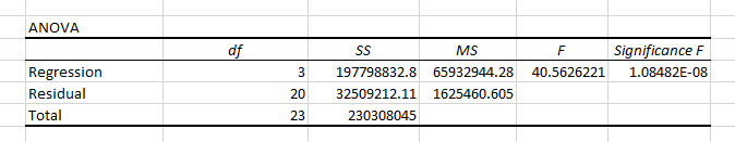
• Regression
  • SS: Sum of Squares of of Regression (or explained) = Σ _i (Yhat_i – Ybar)²
• Residual
  • SS: Sum of Squares of Residual (or error)  = Σ _i (Y_i – Yhat_i)²
• Total
  • SS: Residual (or error) sum of squares + Regression (or explained) sum of squares. Σ _i (Y_i – Ybar)² = Σ _i (Y_i – Yhat_i)² + Σ _i (Yhat_i – Ybar)²
• F
  • F-test with H₀: β₂ = 0 and β₃ = 0 versus H_a: at least one of β₂ and β₃ does not equal zero.
  • Excel computes F as: F = [Regression SS/(k-1)] / [Residual SS/(n-k)]
  • K: Number of regressors including the intercept, n: number of observations
• Significance F
  • Associated P-value for the F-test
  • In our case, Significance F is much smaller than 0.05, then we don’t reject the null hypothesis. This means that all of regressors in our model are significant and their coefficient is nonzero.

Regression Coefficients

This is the component of most interest and reference.

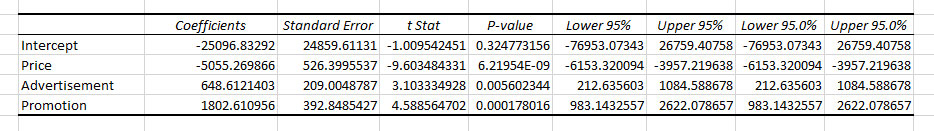
• Coefficients
  • Intercept: The value of Y, the dependent variable when all independent variables equal 0. In our example, the intercept would be the Unit Sales when Price, Advertisement, and Promotion are zero. Here, the value of intercept doesn’t make much sense since it is a negative value, and there is no such thing as a zero Price.
  • Price: The amount we expect the Unit Sales (Y) to increase or decrease per one unit increase in Price (x1). The negative value of Price indicates that with a 1$ increase in Price, Unit Sales will decrease by -25097.
  • Advertisement: The amount we expect the Unit Sales (Y) to increase or decrese per one unit increase of Advertisement (x2). The positive value of Advertisement indicates that with 1$ of increase in Advertisement, Unit Sales will also increase by 649.
  • Promotion: The amount we expect the Unit Sales (Y) to increase or decrese per one unit increase of Promotion (x3). The positive value of Promotion indicates that with 1$ of increase in Promotion, Unit Sales will also increase by 1803.
• Standard error
  • The standard errors (i.e.the estimated standard deviation) of the least squares estimates b_j of β_j.
• t Stat
  •  t-statistic for H₀: β_j = 0 against H_a: β_j ≠ 0.
  • It is divided by the standard error. It is compared to a t Stat with (n-k) degrees of freedom.
• P-value
  • Gives the p-value for test of H₀: β_j = 0 against H_a: β_j ≠ 0.
  • This equals the Pr{|t| > t-Stat} where t is a t-distributed random variable with n-k degrees of freedom and t-Stat is the computed value of the t-statistic given in the previous column.
  • This p-value is for a two-sided test. For a one-sided test divide this p-value by 2 (also checking the sign of the t-Stat).
  • In our case the p-value of Price, Advertisement, and Promotion are less than 0.05 (considering 95% confidence interval), meaning that all these factors contribute to the Unit Sales level. This is not the case for the Intercept, which aligns with our conclusion about Intercept in the Coefficient section.
• Lower 95% and Upper 95%
  • Define a 95% confidence interval for β_j.

 

 

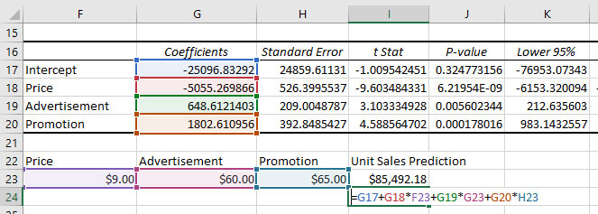
Prediction Using Linear Regression in Excel

A simple summary of our linear regression output is that the fitted line is:

Unit Sales = -25096.83 + 5055.27 * Price + 648.61 * Advertisement + 1802.61 * Promotion

With the regression equation, we can now predict the Unit Sales based on Price, Advertisement, and Promotion.

 

Limitations and Considerations

• Linear regression model assumes a linear relationship and does not account for other potentially influential factors.
• Always consider the context and other variables that may impact the results.

 

Conclusion

Linear regression is a powerful method used by a wide range of experts, including data scientist, scientists, financial analysts, and business analysts to find the relationship between one dependent variable and one or more independent variables. In this blog we started with the mathematical representation of linear regression and introduced some basic concepts. Then, we went on a real-world scenario along with a dataset and solved the issue using regression analysis in Excel. At the end, we could help the sales manager predict sales using linear regression in Excel.