Sensitivity Analysis in Excel: A Practical Guide

Sensitivity analysis, also known as what-if analysis, determines how different values of an independent variable affect a specific dependent variable under a given set of assumptions. In other words, sensitivity analysis studies how various sources of uncertainty in a mathematical model contribute to the model’s overall uncertainty. Excel provides us with a bunch of tools to perform Sensitivity Analysis very effortlessly. Let’s review the list.

 

Tools for Sensitivity (What-if) Analysis in Excel

Excel has three tools for what-if analysis;

• Data tables
• Scenarios
• Goal-seek

Data Tables and Scenarios use sets of input values to calculate possible outcomes. Goal-seek works differently; it takes a single result and calculates possible input values that produce that result.

In addition to these three tools, you can install the Solver add-in to help you perform What-If Analysis. The Solver add-in is similar to Goal Seek, but it can accommodate more variables.

In this article, we will start with a real-world situation with some challenges and then use the tools introduced in this section to deal with the challenges in a systematic way. The reader of this article is supposed to have a working knowledge of Excel and be familiar with basic math.

Let’s start with introducing Data Tables for sensitivity analysis in Excel.

 

Data Tables for Sensitivity Analysis

Data Table is a way of getting multiple results from a single calculation. Let’s assume you want to get a whole lot of different inputs, put them through a single calculation, and get all the different outputs. That’s exactly what the Data Table will give us. 

Data Tables can be found on the Data tab of the ribbon behind the What-If Analysis drop-down. Excel provides the capability to create both one-variable and two-variable data tables, and we are going to look at an example of each.

Note: Data Tables are different from regular Excel tables.

 

One-Variable Data Table

A one-variable data table lets you vary one input to see how it changes the output. To concretely understand how On-variable Data Tables can help us, let’s present a real-world situation.

Estimating Fixed Expenses

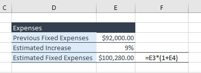
SiSi is a retail company that sells skateboards in the local market. The sales manager needs to make projections about their fixed expenses in the coming year. They have the last year’s fixed expenses and what they think is the likely increase, which is nine percent. They can calculate the Estimated Fixed Expenses using the following Formula:

Estimated Fixed Expenses = Previous Fixed Expenses * (1 + Estimated Increase)

 

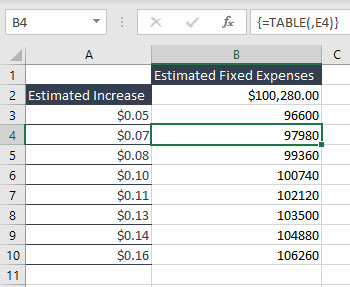
However, the sales manager likes to have a look at a range of different scenarios. Specifically, she wants to see what happens if the likely increase is five percent or how much it will be if it goes up to 14%. That is, she needs the table in the following screenshot to be filled.

 

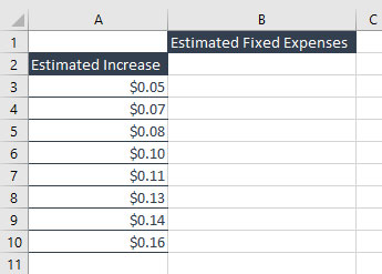
The solution is a One-variable Data Table.

 

Add One-Variable Data Table

1.  Create the formula. 

 

2. Create the data table. 

For this, we’re going to select that whole block. Then we go to Data -> What-If Analysis -> Data Table. The Data Table dialog box offers us two options: Row input cell or Column input cell. In this situation, it’s the column of values we’re changing, not the row. So, we’ll click Column input cell input. 

In the Column input cell, we should select the value in the formula we want to replace with each of the values in the Estimated Increase column. In our case, we want to insert different Estimated Increases in the formula, so we select E4. Click OK, and Excel has completed all the values for us using only one calculation.

 

 

Two-Variable Data Table

Estimating Revenue

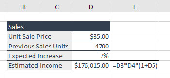
Back to SiSi’s case in the previous section, the next step for SiSi’s sales manager is to make projections about their revenue in the coming year. In their worksheet, they have last year’s sales figures: Unit Sales Price, Previous Sales Unit, and Expected Increase.  They can calculate the Estimated Fixed Expenses using the following Formula:

Estimated Income = Unit Sales Price * Previous Sales Unit * (1 + Expected Increase)

 

What the sales manager is looking to do here is estimate projected revenues depending on the different price points they’ll use for the skateboard and how much they expect their estimated income to go up. That is, she needs the table in the following screenshot to be filled.

 

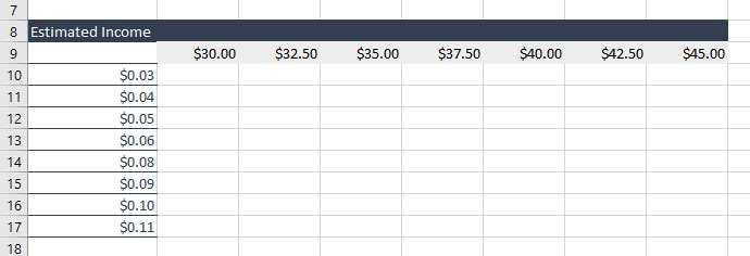
To help the sales manager, we’re going to create a Data Table using two variables so that we can see the different outcomes for the different price points and the different increases. 

 

Add Two-Variable Data Table

1. Create the formula

Make sure that you select the entire block, including the formula. Go to  Data -> What-If Analysis -> Data Table. The Data Table dialog box offers us two options. This time, we have both a Row input cell and a Column input cell. The Row input cell is the value we’re going to swap out using the Sale Price, and the Column input cell is the value that we’re going to replace with Expected Increase. 

Click OK. And that’s our Data Table. A very quick model showing a whole bunch of different options depending on our inputs.

 

Visualizing the Data Table

The best way to visualize a Data Table is by using a heatmap. Excel does not have a heatmap among its charts. So, we resort to Conditional formatting for this purpose.

1. Select the body of the Data Table (Not including the topmost row and the leftmost column)
2. Go to Home -> Styles group -> Conditional Formating -> Color Scales and choose the color scale you like. If you can’t find your favorite color scale, you can choose More Rules to customize the rule and/or the color.

 

More About Data Tables

There are two things about Data Tables we should keep in mind.

• If you click in the Data Table and look at the formula bar, you’ll see it looks slightly unusual. Instead of the normal formula, you’ve got {=TABLE(,E4)}. Whenever you see that, it means we’re dealing with a data table. 

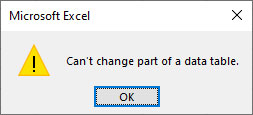
• Another thing to be aware of in Data Tables is if you try to delete just a single cell, Excel will tell you, you can’t change part of a Data Table. It’s a bit of all-or-nothing. If you needed to delete the Data Table, you’d need to make sure you’ve selected all of those results. 

 

 

Scenario Manager

Scenario analysis is a strategic technique that allows users to explore the effects of multiple input combinations on model outcomes. This provides valuable insights into different potential future states. Excel’s Scenario Manager is a powerful tool that facilitates the organization, comparison, and analysis of various scenarios within a single spreadsheet. As usual, let’s begin with a real-world situation.

 

Finding the Optimal Price

Back to SiSi’s case in the previous sections, the sales manager’s next challenge is she is asked to provide some different scenarios for sale price versus quantity sold. 

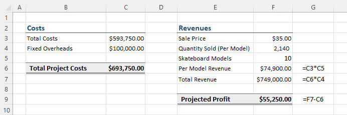
The company has put together a model where they have worked out how many skateboards they hope to produce, the costs involved, and the revenues they hope to make from this. 

The price they are thinking of selling at is $35, and they estimate they will make about 2,140 sales per manual at that price point. If they were to drop the price by $5, research suggests that the quantity sold would go up by 15 percent. On the other hand, if they were to increase the price point by $5, they think it will drop by 15 percent. 

We want to look at what expected projected profit we can get if we were to adjust these two variables: Sales Price and Quantity Sold.

 

 

Before we get into the Scenario Manager, it’s a good idea to name our ranges. It makes life much easier. Now, we want to name two cells: Sales Price and Quantity Sold (Per Model). 

 

 

Adding Scenario

For SiSi’s case, we are going to add three scenarios: Current Price, Increase Price, and Decrease Price.

• Current Price: Sales Price: $35 and Quantity Sold: 2140
• Increase Price: Sales Price: $35 and Quantity Sold: 2140 * (1 – 15%)
• Decrease Price: Sales Price: $30 and Quantity Sold: 2140 * (1 + 15%)

Let’s Add the first scenario: Current Price.

1. Select values of the Current Price and Quantity Sold (not their label).
2. Go to Data tab -> What-If Analysis -> Scenario Manager. The Scenario Manager dialog box will open. At the moment, we have no scenarios because we haven’t added any.
3. Click Add. This will open the Add Scenario dialog box.
4. In the Add Scenario dialog box, select a sensible name for your scenario, and then you’ll notice because we selected F3:F4, they are already selected in the Changing cell box. But if you had not done that previously, you could specify the cells that will change over here. 
5. Click OK, and it shows us the current values in the Changing cell we selected in the previous step. This is exactly the scenario we want to save. 
6. Click OK, and you will go back to the Scenario Manager dialog box with all scenarios listed there.

 

Adding the second and third scenarios is similar.

 

All right, so we’ve created three scenarios, but if you look in your workbook, nothing has changed at this stage. Let’s see how we can make use of these scenarios.

 

Using Scenarios

1. Go to Data -> What-If Analysis -> Scenario Manager, and this will open up the Scenario Manager dialog box. 
2. Now select the Current Price scenario and click Show. Nothing will change. Then select the Increase Price and click Show; you can see that Per Model Revenue, Total Revenue, and Projected Profit will change accordingly. Repeat for the Decrease Price scenario.

 As you can see, the current price is making the highest profit.

3. You can also create a summary of all your scenarios in another worksheet. To do that, you just need to click the Summary button. 

Goal Seek for Sensitivity Analysis

When you know the result of a formula but you’re not sure what input value the formula requires to get that result, you can use Excel’s Goal Seek feature. That is, with Goal Seek, you go from output to input, which is the opposite of what we have in Data Table and Scenario Manager. Let’s go on with the case of SiSi.

Finding the Optimum Quantity to Produce

SiSi’s sales manager has put together a model where they have worked out how many skateboards they hope to produce, the fixed costs involved, and the revenues they hope to make from this.

 

In the Projected Profit, they have a calculation that relies on these inputs, and one of them is the number of skateboards they produce. At the moment, this calculation is producing the answer. What the sales manager wants to do is change the answer to zero by adjusting this input.

Using Goal Seek

1. Click on the value of Projected Profit. 
2. Go to Data -> What-If Analysis -> Goal Seek. This will open the Goal Seek dialog box.
3. A set cell is the cell that contains the calculation we want to change the value it’s returning. Because we selected it beforehand, you’ll see it’s already populated.
4. To value is the value we want to equal, and that is a zero in our case.
5. The final box, By changing cell, is which input we want to change to get to that result. This value must be a typed-in value rather than a formula. 
6. Click OK. Do you see all the numbers changing?
7. We can either accept the solution by clicking OK or if we want to get back to our original, we can click Cancel.

 

Now we know the minimum number of manuals we have to produce, so we don’t make a loss. 

Limitations and Assumptions

While sensitivity analysis is a powerful tool for understanding the impact of input variables on model outcomes, it comes with certain limitations and assumptions that users need to be aware of. Recognizing these limitations is crucial for proper interpretation of results and making informed decisions. Here are some key limitations and assumptions associated with sensitivity analysis:

1. Assumption of Variable Independence:
   • One of the common assumptions in sensitivity analysis is that input variables are independent of each other. In reality, variables are often interconnected, and changes in one variable can influence others. Sensitivity analysis might overlook complex interactions, leading to an oversimplified view of the system. Users should be cautious when interpreting results, especially in scenarios where variables are not truly independent.
2. Linear Relationships:
   • Many sensitivity analyses assume linear relationships between input variables and the model’s output. In reality, relationships can be nonlinear, and the impact of changes may not be proportional. Nonlinearities can lead to inaccuracies in sensitivity analysis results, particularly when variables exhibit complex interactions, diminishing returns, or increased sensitivity at extreme values.
3. Static Nature:
   • Sensitivity analysis often assumes that relationships between variables remain constant over time. In dynamic systems, where conditions and relationships evolve, this assumption may not hold. For instance, market dynamics, consumer behavior, and external factors can change, impacting the sensitivity of the model to different variables. Sensitivity analysis results may provide a snapshot but may not capture the evolving nature of the system.
4. Limited Scope of Analysis:
   • Sensitivity analysis typically focuses on a predetermined set of input variables, potentially overlooking unforeseen factors that may influence outcomes. This limitation emphasizes the importance of a comprehensive understanding of the model and the external environment to ensure that the analysis covers all relevant variables.
5. Deterministic Nature:
   • Sensitivity analysis is often deterministic, meaning it provides insights based on specific values or scenarios. This might not fully capture the probabilistic nature of uncertainties. In situations with inherent randomness, probabilistic sensitivity analysis (PSA) or Monte Carlo simulations may be more appropriate to account for the stochastic nature of variables and outcomes.
6. Static Model Structure:
   • Sensitivity analysis assumes a fixed model structure during the analysis. Changes to the model’s structure, such as the addition of new variables or alterations to the underlying equations, may impact the results. Users should be aware that sensitivity analysis results are contingent on the model’s structure at the time of analysis.

Importance of Recognizing Limitations

Recognizing the limitations and assumptions of sensitivity analysis is essential for accurate interpretation and effective decision-making. Users should exercise caution in generalizing results and be aware of potential biases introduced by these assumptions. Incorporating a degree of uncertainty into the interpretation allows decision-makers to develop more robust strategies that account for the inherent complexities of real-world systems.

Conclusion

In conclusion, sensitivity analysis in Excel is a valuable technique that allows individuals to assess the impact of variable changes on their financial models and decision-making processes. Through the examples provided in this ultimate guide, we’ve explored two powerful tools: creating one-variable data tables and using Goal Seek.