Excel Function List: 10 Commonly Used Functions in Excel

Excel is a useful tool for everyone, from making a simple list to doing complicated math, there is nothing you can’t do on this handy application. Among all the options that this tool has, Excel functions are the most useful ones because they let you create your form or analytical report more interactive and accurate. Here is the list of the most common Excel functions.

10 most used Excel functions

Here’s a list of 10 most used Excel functions

Excel Count Function 

If you want to know how many cells contain data in your spreadsheet, you can use the COUNT function. However, you should know that the simple COUNT function only checks the cells for numeric data, so if the cells contain text or formula, they’ll not be counted.

To count all the cells in a range containing any type of data (text, numbers, formula, etc.), you can use the COUNTA function, which counts all the cells except the blank ones.

In case you are looking to count the blank cells, the blank cells, you can use the COUNTBLANK function.

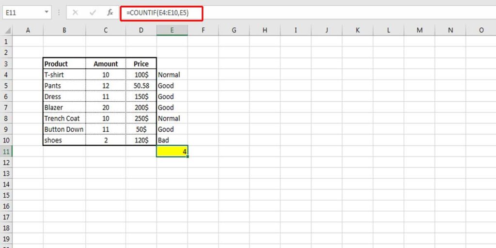
There is another counting function which helps you count the cells that have a specific condition. Using the Excel COUNTIF function, you can set a condition and count specific cells having that condition. For example, you want to know how many cells contain a particular text such as “Good”, or how many cells have numbers that are higher than “7”. So, you have two parts in this type of function, one specifies the range and the other specifies the condition. The formula will be as follow:

The result of all types of count functions will be a number, which will be displayed on the cell that contains the formula.

Please note that the COUNT function is different from the SUM function, which will be explained next. 

Excel SUM Function

One of the most common and frequently used functions in Excel is the SUM function, which helps you easily calculate the numeric data in cells. The simplest way to calculate numbers in a row or a column is by clicking on AUTOSUM on the Home tab. However, it’s also possible to calculate numbers that are in different rows using the SUM formula and “+” sign, check out the following formula:

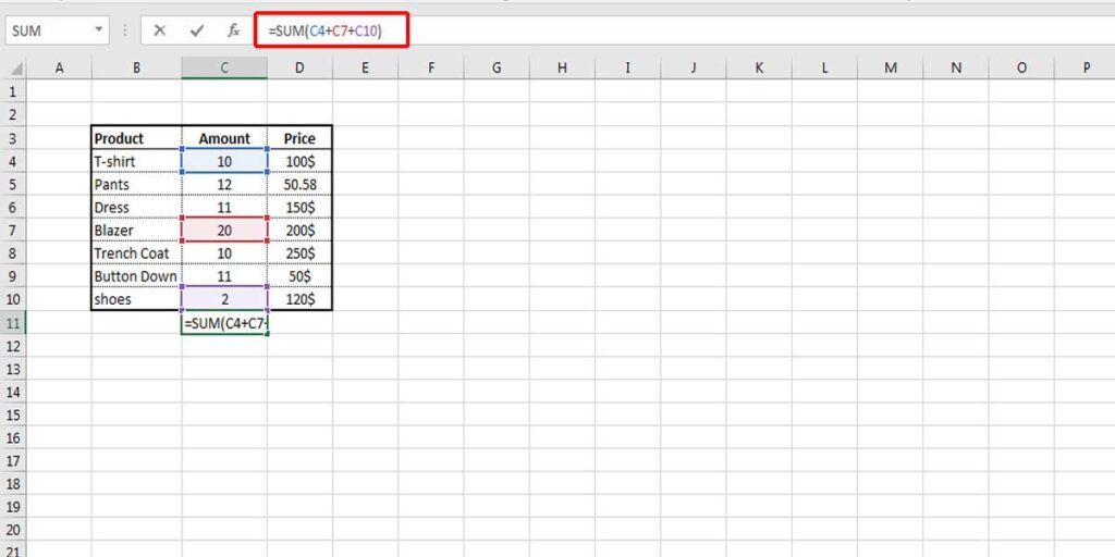
In this method, you only need to select the cells that you want to calculate.

Excel AND Function

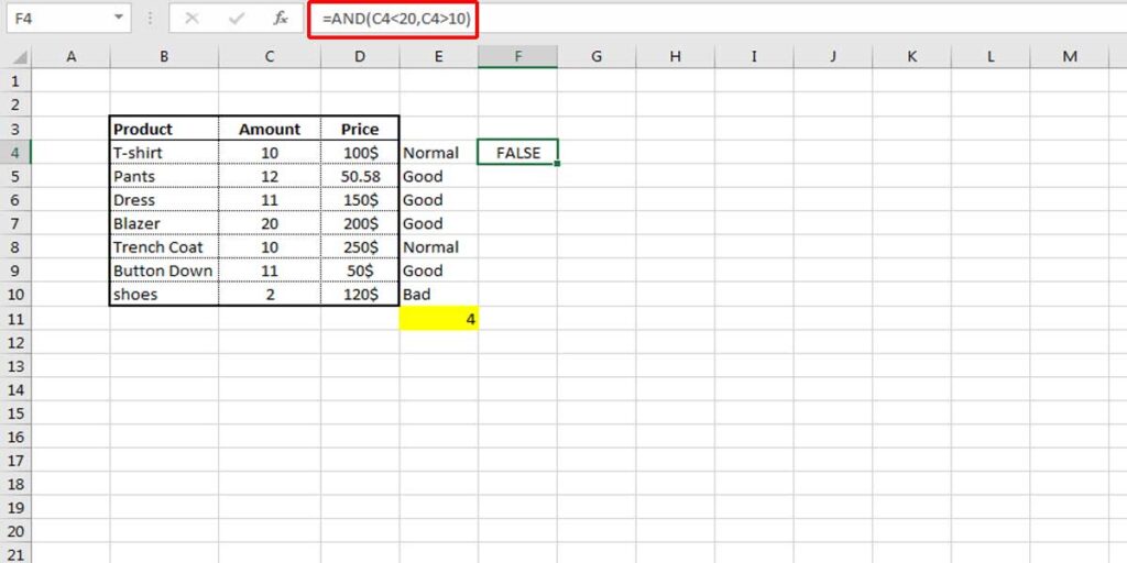
AND function is a logical function that checks multiple statements. If all conditions are TRUE, it will return “TRUE”, but even if one condition is false, the result will be “False.” Check the following statement:

AND (A2>10, A2<20)

It means it returns TRUE if A2 is 15, but it will return FALSE if it is 21.

AND function can be used in combination with other functions such as OR, IF. Since it can check multiple conditions, it’s mostly like the IFS function and they can be used interchangeably. So, if your version of Excel is old and you don’t have an IFS function, you can use the AND function as the logical test inside the IF function to avoid extra nested Ifs.

Average Function

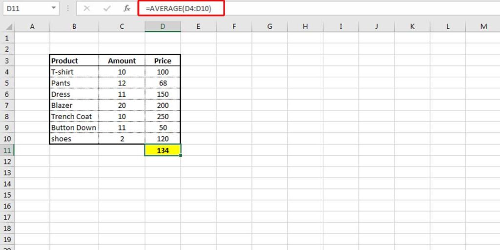
This is one of the extremely useful and also simple tools which helps you find the average value between a range of numbers. The function has several functions in its heart because generally finding the average value needs various processes. Usually, the numerals are calculated first and will be divided into the number of cells. But, with the Average function, none of the steps are needed because it does all the steps in a blink of an eye.

Like all other Excel functions, the AVERAGE function starts with an “=” sign in the cell or the address bar. Then you can add the formula by writing the word AVERAGE and opening parenthesis. The AVERAGE function needs two or a range of values, which can be selected in the spreadsheet. Check the following example:

The AVERAGE function also has different types which are AVERAGEIF, AVERAGEA, and AVERAGEIFS. 

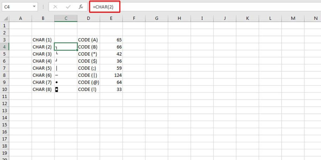
CHAR Function

This function has a more complicated usage. It receives a number and returns a character. Generally, each character has a numerical code between 0-255. Therefore, the CHAR function turns ASCII code into its characters. This function is used for characters that are hard to enter into a formula.

The opposite side of the CHAR function is the CODE function, which receives the character and returns its CODE, such as the following example:

IF and IFS Functions

One of the reasons that make Excel so wonderful is because you can check cells for different conditions. Up until 2016, you could only use the IF function, which checked only two conditions that had a TRUE or FALSE result. For example, it was only possible to check if the data in the cell is greater than 10.

In the latest versions of Excel, from its 2016 version onwards, Excel introduced a new conditional function called the IFS function. Now it’s possible to do more complicated conditions using the IFS function. For example, to check if the data is greater than 10 and at the same time smaller than 20. Therefore, the result will only return data in this range. In fact, the IFS function can have more than two conditions, it covers up to 127 statements.

MATCH Function

The MATCH function can help you find a certain value in a range of cells and return its position. This function has three sections; the first is the value you want to find and its match, which is usually a text. Second, you need to mention in which cells you want to find that match, which can be done by selecting the range of cells. The last part is the match type, which means you want to find the exact match or the closest match. It can be 1,0 or -1. The most frequently used option is 0, which is used to look for the exact match. Let’s see the result in the following example:

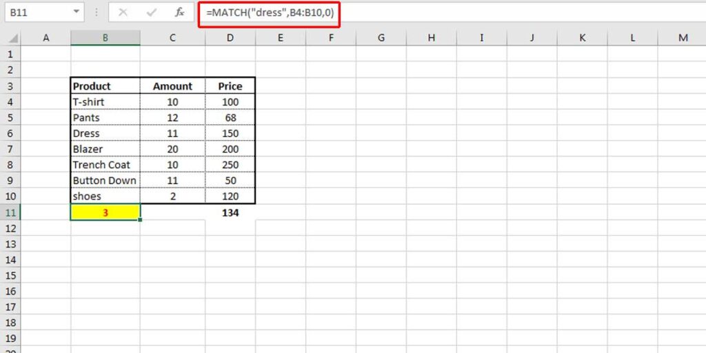
The result is 3, which means the exact match for “dress” is found on the third cell between B4 to B10. 

VLOOKUP Function

One way to search for a value in a column and return a value from a different column in the same row is using the VLOOKUP function. Consider you have a table of your products,their prices and number of items sold, you want to find the price of one of the products. VLOOKUP helps you write a formula that can do this search for you. VLOOKUP stands for Vertical Lookup, which means, it does the search in vertical form (or in the column you mention in the formula). Let’s see the formula below and the result it returns.

If you intend to use this function on larg data you might find this blog interesting: How to Handle Large Excel Files with vLookup Formulas Referring to Other Workbooks

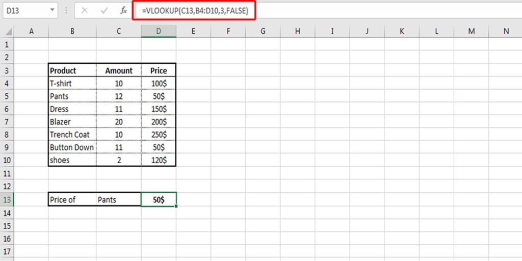
In this simple example, we want to know the price of a product, so we write it in a separate cell. Then, we write the formula using VLOOKUP in another cell. VLOOKUP contains different parts, first, we need to mention the cell we want to read its value, in this example, it’s C13. Next, the range that we want to read and find the mentioned value should be selected, in this example, it’s the whole table from B4 to D10.

In the next part of the formula, we need to make it clear which column should be read. In our example, it’s the third column of the range that has been selected. If we want to find the Amount, we need to input 2 instead of 3. Then we have TRUE and FALSE, which are used when we want to read the Exact Match or Approximate Match of the value,as you can see above the result is $50. 

ROUND Function

Rounding numbers is a common function in Excel, especially when we do calculations that might have some decimal digits. There are different types of rounding a number in Excel, which is under the ROUND group. The simple ROUND function can round the mentioned number or the value in a cell to the specific number of decimal places. For example, if the number has two decimal places, we can round it to one, which means the number should have one decimal place so it will be rounded to the nearest number. See the following example:

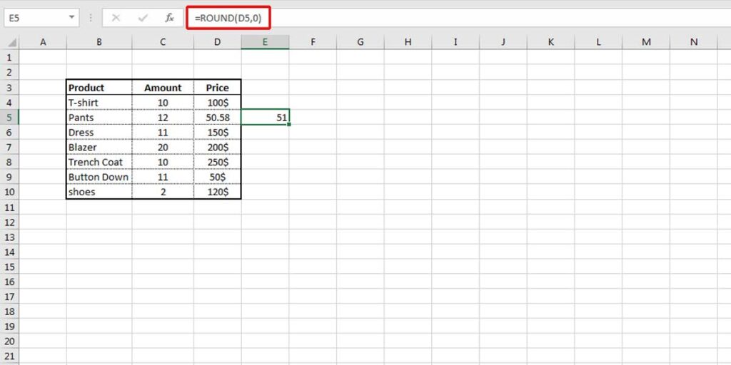
In this example, we have rounded the number in D5 to 0. It means, we don’t want the result to have any decimal number so it will be rounded to the nearest number, which is 51. The positive numbers will round up the numbers and the negative numbers will do the opposite. There are other rounding options in Excel, the most common ones are ROUNDUP, ROUNDDOWN, MROUND.

CONCATENATE Function

This function is used to gather the values of different cells together and return them to a different cell. CONCATENATE function is very simple yet very effective because it can combine several columns or fields. Assume you have a table of your customers’ addresses, which have been separated into different cells. You can combine the information of each cell to make a complete address. Let’s check that in the following example:

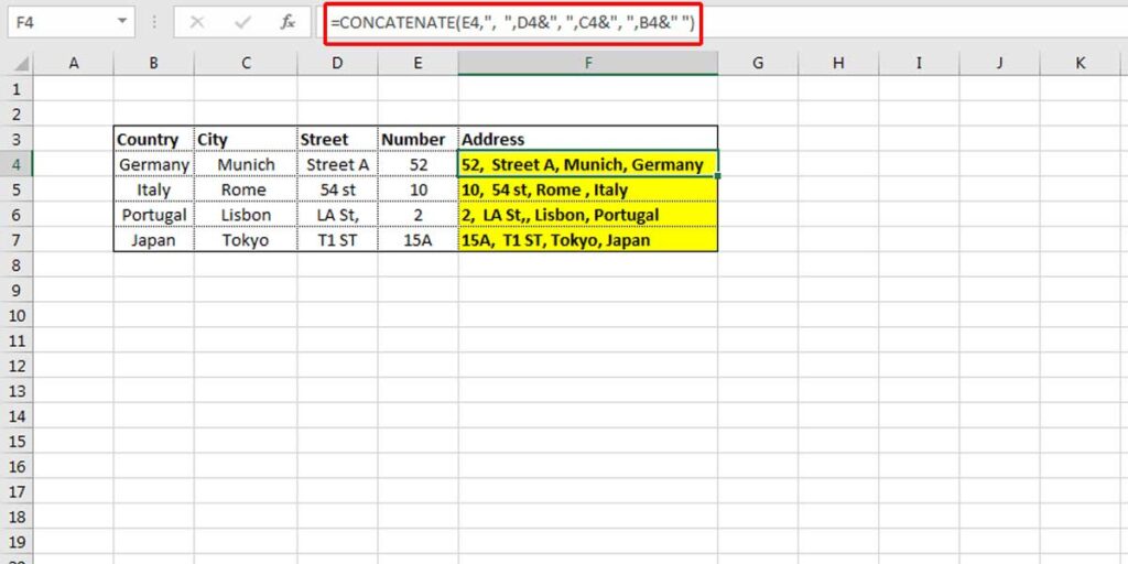
You only need to add a SPACE between each cell so the values won’t stick together and become more clear to read. 

Bottom Line 

Excel has a handful of functions that are used in different situations. Some are more commonly used, while others may have more advanced uses. It would be extremely helpful if you learn to use the more basic and frequently used Excel functions so that you can easily improve your overall business productivity.