How To Add Axis Labels In Excel Charts

Charts are essential for visually representing data, but without clear labels, they can be confusing. In our mission to share Excel tips and tricks, we want to emphasize how to add axis labels in Excel.

Axis titles and labels are crucial for providing clarity and context to chart data. They help interpret chart data more effectively by explaining what the X and Y axes represent.

For instance, the X-axis might indicate time, while the Y-axis could represent sales figures. In some cases, you may even need to show two different scales on the same chart — learn how to add a secondary axis in Excel to visualize such comparisons more effectively. It’s also important to differentiate between axis labels and axis titles.

If you’re exploring different ways to visualize data, check out our Waterfall Charts in Excel: A Complete Tutorial. It’s a great next step for understanding how to show increases and decreases clearly in your datasets.

In this guide, we will walk you through how to add, modify, and distinguish between axis labels and titles in Excel charts. Stay tuned!

Why Are Axis Labels and Titles Important?

Before we get into the steps, it’s crucial to understand why axis labels are important in Excel charts. Axis labels provide context for the data being displayed.

They indicate what each axis(X and Y) represents, making it easier for users to interpret the information. This is especially helpful when sharing charts with stakeholders or team members who may not be familiar with the data.

Consider a chart displaying sales data over several years. Without axis labels indicating “Year” on the x-axis and “Sales (in $)” on the y-axis, viewers may misinterpret the data or fail to understand its significance.

Proper labeling enhances clarity and aids in effective data visualization. Without clear labels, the audience may struggle to understand what the data represents which may lead to potential misinterpretation.

Keep reading to learn how to insert axis labels and titles in Excel charts.

What Are Axis Labels in Excel?

Before diving into the details of how to add x and y axis labels in Excel, let’s first understand what axis labels are.

In the charts you create, axis labels appear beneath the horizontal (category or “X”) axis, alongside the vertical (value or “Y”) axis, and next to the depth axis in a 3-D chart.

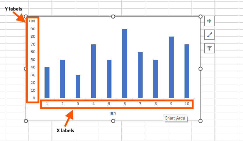
In a chart you create, axis labels are positioned as follows:

• Horizontal Axis (X-Axis): Axis labels are displayed below the horizontal axis. These labels typically represent categories or discrete data points, such as time intervals or specific items.
• Vertical Axis (Y-Axis): Axis labels appear next to the vertical axis. They usually denote values or measurements that correspond to the data points plotted on the chart.

Note: For 3-D charts, an additional depth axis may be present, complete with its own set of axis labels positioned accordingly.

Axis labels in your chart are directly derived from the source data used to create it. This means that any changes made to the underlying data will automatically update the corresponding axis labels in the chart.

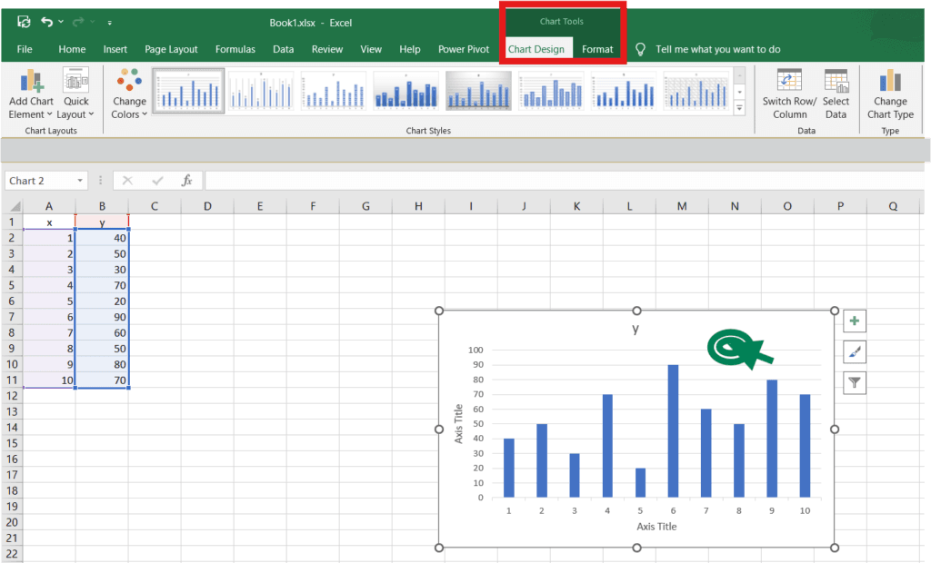
How to Make the Axes Labels Appear on the Chart

At first, the axes may not appear on the chart. If your chart doesn’t display axes by default, you can easily make them appear.

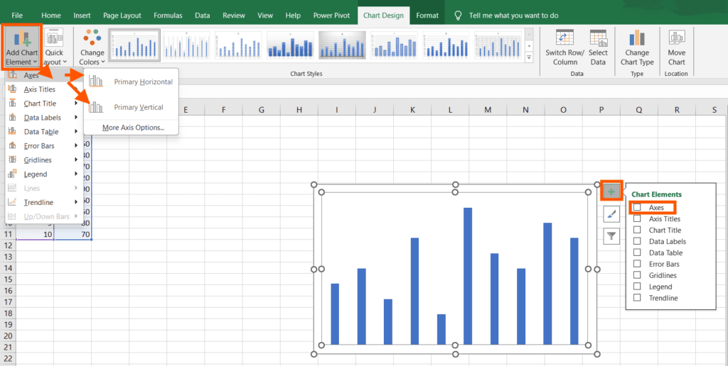
There are two paths to enable axis labels. To do so, follow these steps:

Path 1: Enabling Axes Through Chart Elements

1. Select the Chart: Click on the chart to activate it.
2. Open Chart Elements: Click the “+” button or “Add Chart Elements” option.
3. Check the “Axes” Box: This will enable both the horizontal (x-axis) and vertical (y-axis).

Path 2: Enabling Axes Through Chart Design

1. Select the Chart: Click on the chart to activate it.
2. Go to the “Chart Design” Tab: This tab appears in the ribbon when a chart is selected.
3. Click on “Add Chart Element”: A dropdown menu will appear.
4. Select “Axes”: This will enable both the horizontal (x-axis) and vertical (y-axis).

Once the axes are visible, you can either change the axis labels(by changing the data) or add titles to provide context for the data. Keep reading to learn how to edit axis labels in Excel.

How to Change Axis Labels in a Chart

As we said, axis labels derive their text from the source data in your worksheet. So, to change axis labels you need to change the data.

To change the text of the axis labels in Excel, follow these steps:

• Select the Cells: Click on each cell in your worksheet that contains the label text you want to modify.
• Edit the Text: Type the new text for each label in the respective cell and press Enter.
• Automatic Update: As you change the text in these cells, the corresponding labels in your chart will automatically update to reflect your changes.

How to Make Label Text Different from Worksheet Labels

If you want the labels to differentiate from the data you inserted, you can change them. To create custom labels in the chart that are independent of the worksheet data:

1. Right-click on the category labels you want to change and select Select Data.
2. In the Horizontal (Category) Axis Labels box, click Edit.
3. In the Axis label range box, enter your desired labels, separated by commas. 

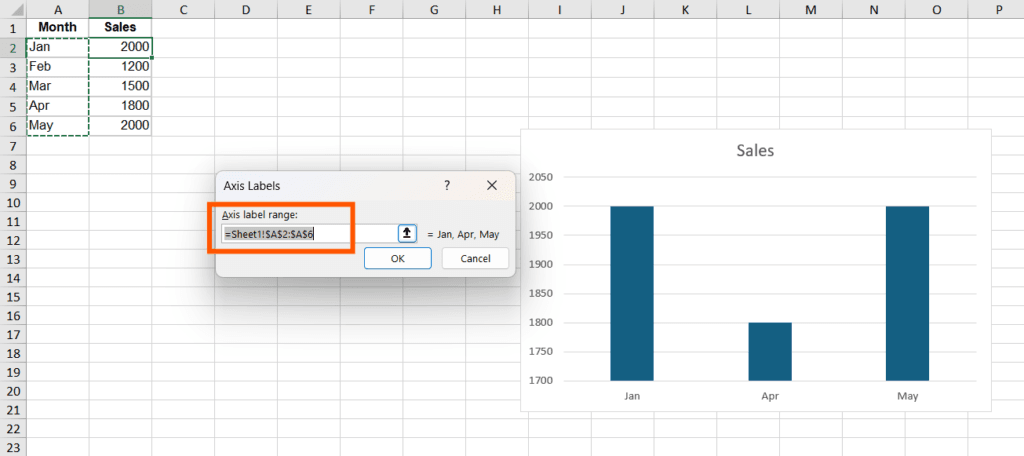
This method allows you to have distinct labels in your chart that do not alter the underlying data in your worksheet. This provides flexibility in how you present your information.

How to Change the Format of Text and Numbers in Labels

To format text and numbers in Excel chart labels, follow these steps:

1. Right-click on the category axis labels you wish to format and select Font.
2. In the Font tab, choose your preferred formatting options.
3. To adjust character spacing, click the Character Spacing tab and select your desired spacing options.

Changing Number Format:

1. Right-click on the value axis labels you want to format and select Format Axis.
2. In the Format Axis pane, click on Number.
   • Tip: If you don’t see the Number section, ensure that you have selected the value axis, which is typically located on the left side.
3. Choose the format options you prefer. If your selected format includes decimal places, specify the number of decimal places in the Decimal places box.
4. To keep the numbers linked to the worksheet cells, check the Linked to Source box.

Note: Before formatting numbers as percentages, ensure that the numbers displayed on the chart have been calculated as percentages in the worksheet or are represented in decimal format (like 0.1). For example, if you enter =10/100 in the worksheet and format the result 0.1 as a percentage, it will display correctly as 10%.

Adding axis labels to your Excel charts helps provide context for the data by labeling each axis. Now let’s discuss the Axis titles.

What Are Axis Titles in Exel?

Axis titles in Excel charts indicate what the x-axis and y-axis represent, acting as crucial aids for data interpretation. They function similarly to labels for the X and Y axes, which often leads to confusion between titles and labels in Excel.

These titles provide essential context for the plotted values. This enables viewers to quickly comprehend the relationships between different variables. By clearly stating what each axis represents, axis titles improve the clarity of your charts.

Limitations on Axis Titles: Note that you can only name axes in charts that include them already. For example, pie or doughnut charts have no X or Y axis, so they can’t be named.

Axis titles may not shown automatically in a chart. To add axis titles and describe what is represented on the axis, refer to the following instructions.

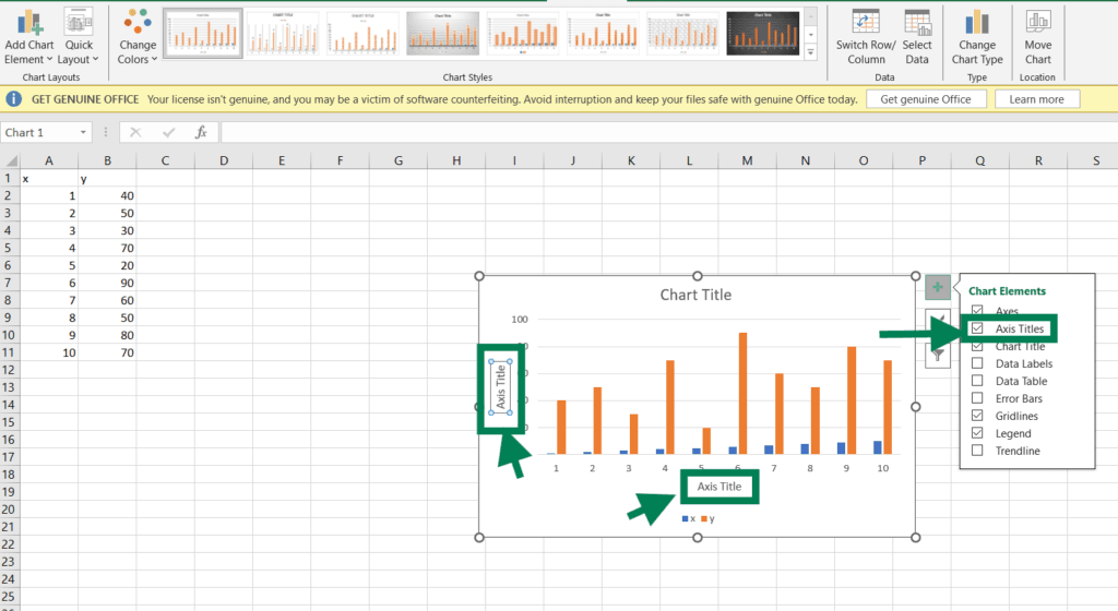
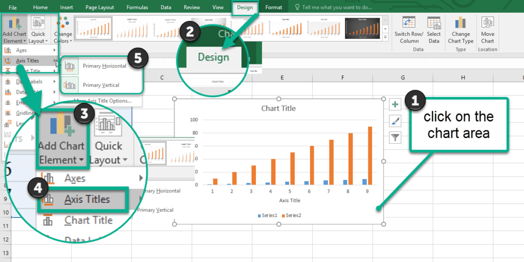
Method 1- Add Axis Title by The Add Chart Element Option

When you create an Excel chart, both horizontal and vertical axes don’t have titles.

To add the axes titles for your chart, follow these steps:

1. Click on the chart area to select the chart.
2. Go to the Design tab from the ribbon.
3. Click on the Add Chart Element option from the Chart Layout group.
4. Select the Axis Titles from the menu. 
5. Select the Primary Vertical to add labels to the vertical axis, and Select the Primary Horizontal to add labels to the horizontal axis.

Once the axis titles are enabled, click on the axis title text box that appears on your chart. Then type your desired axis label. For example, for the X-axis, you might enter “Months,” and for the Y-axis, “Sales ($).” After typing your label press Enter.

Method 2- Add Axis Title by The Chart Element Button 

Excel 2013 and later versions provide a useful cross-cut, which is shown by a plus element. 

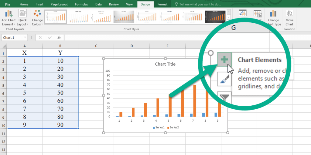
Use this button to add titles to your chart axes:

1. Click on the chart area.
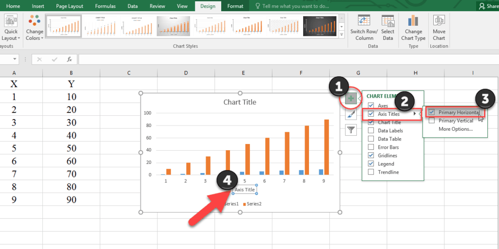
2. Click on the Chart Element button (according to picture 2.)
3. Check the Axes Titles from the checklist (if you need to add a label to one of the axes, click on the little arrows in front of the Axes Titles checkbox and check the Primary Vertical or the primary Horizontal checkboxes.)
4. Enter the axis title.

Enhance your software capabilities with our customizable Add-In Solutions, seamlessly integrating new features to meet your business needs.

Dynamic Axis Labels: Linking Axis Titles to Cells

You can create dynamic axis labels by linking the axis titles directly to cells in your worksheet. This ensures that any updates to your data are automatically reflected in your chart labels. So, you can save time and improve consistency across updates.

Let’s see how to link the chart axis name to the text we already mentioned in a workbook.

1. Add Title one of your chart axes according to Method 1 or Method 2.
2. Select the Axis Title.

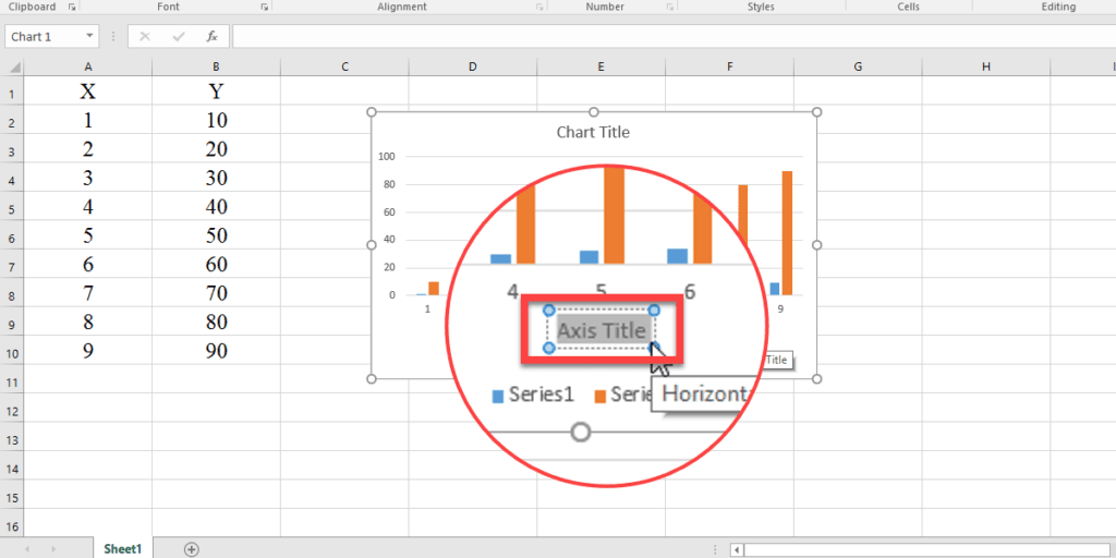
3. Click in the Formula Bar and enter =.
4. Select the cell that shows the axis label. (in this example we select X-axis)
5. Press Enter.

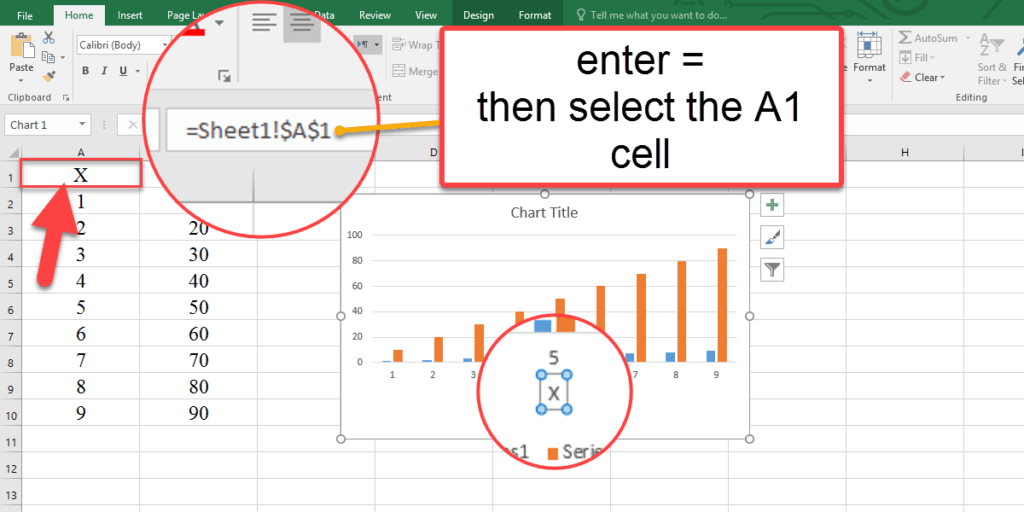
When you click in the Formula Bar and enter =, then select the cell that contains the desired axis label (in this example, the X-axis), and press Enter, you are dynamically linking the axis title to that specific cell.

This action has the following effects:

• Dynamic Updates: The axis title will automatically update if the content of the linked cell changes. For example, if you update the cell to reflect new data, the axis title will reflect the change without needing manual adjustment.
• Consistency: It maintains consistency and is particularly useful when working with large datasets or frequently changing information.
• Automation: This method reduces the need for manual edits in the future, saving time and minimizing the risk of errors when updating the chart.

Video 1- Link the chart axis name to the text

How BSuite365 Help

Properly labeling your charts is crucial for effective data visualization, and BSuite365 specializes in optimizing this process to enhance your data presentation.

BSuite365 offers expert Excel consulting services designed to optimize your data management and enhance productivity.

Our team specializes in transforming complex data into actionable insights, ensuring you harness the full potential of Excel for your business needs.

You can connect with us and ask our experts for your inquiries and get more Excel Support Services.

Why BSuite365?

• Expert Guidance: Our consultants can help you navigate the nuances of Excel, ensuring that you not only add axis titles correctly but also customize them for maximum impact. Whether you’re using the Chart Elements button or the Design tab, we provide tailored support to streamline your chart creation process.
• Advanced Customization: As highlighted in the article, linking axis titles to specific cells can make your charts dynamic. BSuite365 offers advanced solutions that automate these processes, allowing your charts to update in real-time as your data changes.
• Comprehensive Training: We understand that many users may struggle with formatting and positioning axis labels. Our training sessions cover everything from basic label addition to more complex formatting options, ensuring you feel confident in using Excel’s full capabilities.
• Efficiency Improvements: Just as the article emphasizes the importance of clear labeling for data interpretation, our services focus on enhancing your overall efficiency. We help automate repetitive tasks and improve your workflow, allowing you to focus on analyzing data rather than formatting charts.

Reduce costs, accelerate tasks, and improve quality with Excel Automation Services.

Formatting and Customizing Axis Titles

To enhance the readability of your charts, you can format axis titles by adjusting the font style, size, color, and even rotation. This helps make the information clearer and more professional-looking.

Advanced Formatting Tips:

1. Rotate Axis Labels: If your axis labels overlap or are too long, you can rotate them for better legibility. Right-click on the axis labels, select “Format Axis”, and adjust the “Text Direction” or “Angle” to rotate the labels.
2. Change Font Style, Size, and Color: Right-click on the axis title, select “Font”, and customize the appearance by choosing a new font, adjusting the size, or changing the color to match your chart’s design.
3. Include Units of Measurement: For added clarity, include the units of measurement in the axis titles. 

By applying these formatting techniques, you can make your charts not only more visually appealing but also more informative and easier to interpret.

Troubleshooting Common Issues

When editing or adding axis labels in Excel, you may encounter some common problems. Here are two frequent issues and their solutions:

Axis Titles Not Appearing:

• Check Chart Type: Ensure that the chart type you are using supports axis titles. For example, pie charts and doughnut charts do not have axes, so axis titles cannot be added.
• Verify Chart Elements: Make sure that the “Axis Titles” option is selected under the Chart Elements menu (the green plus (+) icon next to the chart). If it is unchecked, enable it to display the axis titles.

Incorrect Formatting or Positioning:

• Overlapping or Misaligned Labels: If the axis titles or labels overlap or are misaligned, you can adjust their position using the “Text Direction” and “Text Alignment” options found under the Format Axis Title menu.
• Manual Adjustment: You can also manually drag the axis titles within the chart area to reposition them more effectively, ensuring they do not interfere with the data or other chart elements.

By following these troubleshooting steps, you can resolve common issues and enhance the appearance of your Excel charts. This will help ensure that your data is presented clearly and effectively.

Conclusion on Axis Titles and Labels

Properly labeled charts are crucial for effective data visualization, as they significantly enhance the clarity and interpretability of information. 

Well-defined axis labels and titles provide essential context, allowing viewers to quickly grasp the relationships between variables and draw meaningful insights from the data presented.

By taking the time to customize and troubleshoot your chart labels, you not only improve the visual appeal of your charts but also ensure that your audience can accurately understand and engage with the information.

For those looking to elevate their Excel skills further, exploring advanced chart features can unlock new ways to represent data effectively. Additionally, seeking professional consultation can provide tailored guidance and support, helping you maximize the potential of Excel for your specific needs. 

Enhance your business efficiency with our specialized Macro Development Services, tailored to automate and streamline your operations for maximum productivity.