How To Sum In Excel
Knowing how to add and sum is fundamental when it comes to working with Excel. In our previous blog “How To Add Numbers, Cells, And Columns In Excel”, we guided you through basic ways to add numbers, cells, and columns. We also mentioned the basics of the Sum formula. In this tutorial, we are going to cover other methods known as AutoSum and the SUM function.
Excel offers various mathematical functions, and while summing values is one of the most basic operations, learning how to divide numbers in Excel is equally essential. If you’re interested in mastering division, check out our detailed guide on How to Divide in Excel.
Before we dive into the various ways to sum data in Excel, it’s worth noting that Microsoft Excel has undergone several updates in recent years. For instance, Excel 2016 introduced some exciting new features, including changes to functions and features that can make your calculations more efficient. If you’re curious about these updates, check out our blog on what’s new in Excel 2016.
How to use AutoSum to add in Excel
Basically, if you want to add adjacent cells, columns, or rows, you can use AutoSum which is the quickest way.
How to total a column in Excel
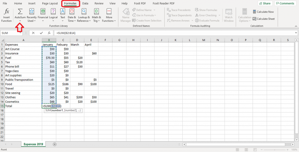
Here is how you use AutoSum to add the values in a column:
- Click on the cell below a column of adjacent cells
- Go to the Formula tab, click on AutoSum
- Press Enter, Excel adds all of the adjacent cells
In the screenshot below, cell B15 is the last cell below the column.
Boost your productivity by getting a free consultation from Excel experts, and discover tailored solutions to optimize your data management and analysis.
How to sum a row in Excel
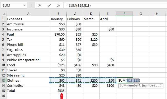
As mentioned above, you can add the values in adjacent rows, as well.
- Click on a cell right of the row of adjacent cells
- Click on AutoSum by going to the Formula tab
- Press Enter and the cell displays the results
If you look at the screenshot you can see that cell F13 is the last cell to the right of the row.
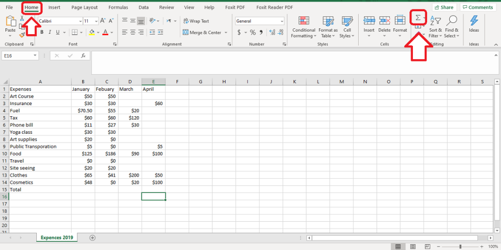
You can also find AutoSum by clicking on the Home tab in the Editing section. The shortcut for AutoSum is [Alt+=].
How to get the grand total in Excel
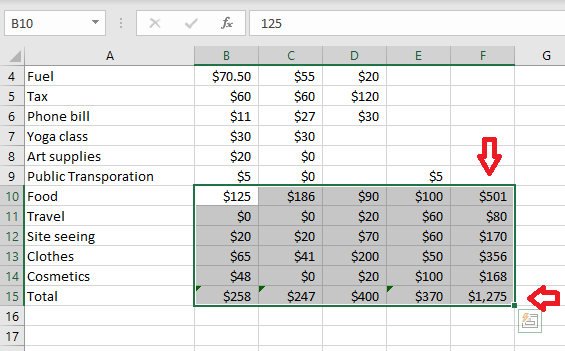
If you want to get the sum of the rows and columns, including the grand total, follow the steps below.
- Select a group of adjacent cells and an extra (blank) column and row.
- Go to the Home tab in the Editing section.
- Click on AutoSum and get the sum of the rows and columns, including the grand total in the extra column and row you have selected.
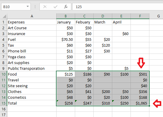
Bear in mind, if you update any of the cells with new values or figures, AutoSum will automatically update the results in each row and column, including the grand total. You can compare the screenshot below with the one above to see how the data updates have changed the AutoSum results.
Enhance your software capabilities with our customizable Add-In Solutions, seamlessly integrating new features to meet your business needs.
How to use the SUM function in Excel
The SUM function in Excel is another option for adding values. Remember that a function is just a predefined formula. You must also be aware that you can use up to a total of 255 individual arguments. These arguments include numbers, cell references, ranges, arrays, and constants, or a mix of all.
Here is a simple example which shows how the SUM function works.
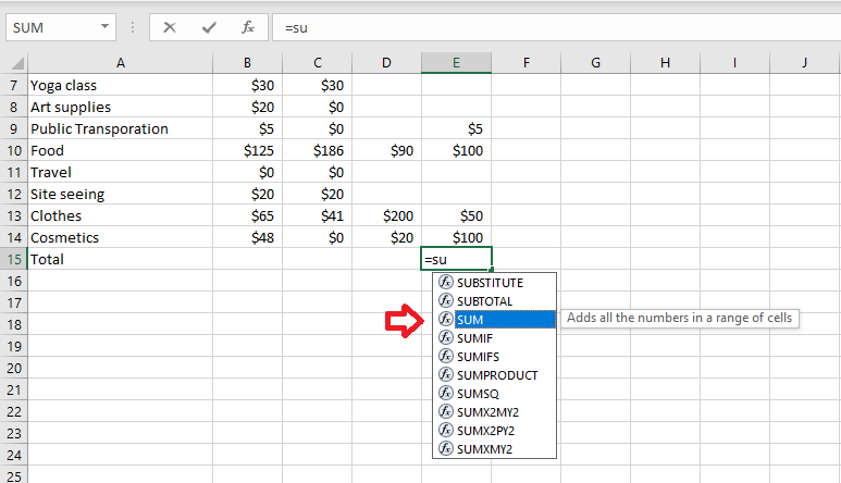
- Click on an empty cell where you want to see your SUM function results.
- You can either start with typing =SUM( manually, or as you start typing =SUM you will see a box appear below the cell, double click on SUM or press Tab, and the formula will appear.
- Now that you have the formula, hold down the Ctrl key, select the range of cells you want
- Press Enter to finalize the function and see the results
Again, if you look at the screenshot, you can see the range of cells that are selected in the cell and in the formula bar. In the next paragraph, you can check out the description provided for the SUM function formula.
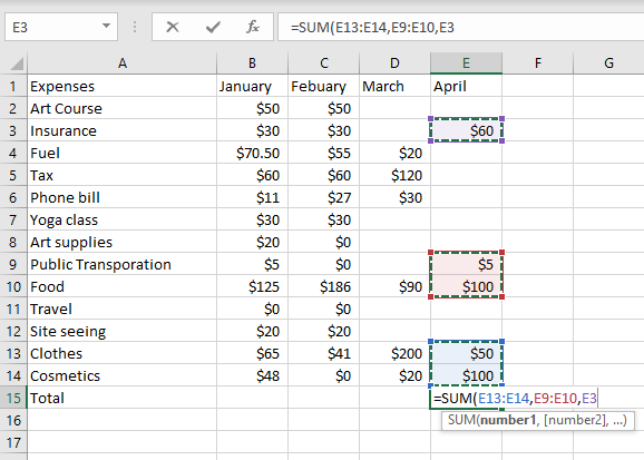
This SUM function starts with an = sign, then the SUM function, open parenthesis, then the first range of cells, E13:E14 (this is the number1 argument in the SUM function), then a comma, then the next range of cells, E9:E10 (this is the number2 argument in the SUM function), and then the last cell reference E3 (this is the number3 argument in the SUM function), then the closing parenthesis. The next screenshot demonstrates the final result.
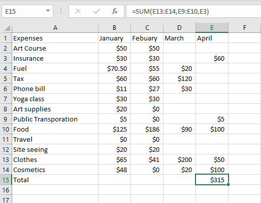
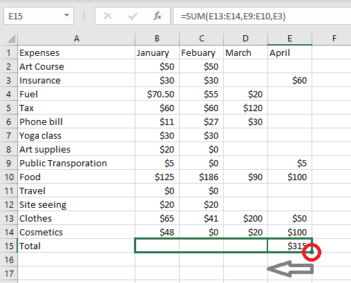
- Now that you have the results based on the SUM function, you can fill in the adjacent cell with the same formula, so you click on the cell that has the results and point your cursor to the right-bottom corner and it will change to a black sign. Now, press hold and drag towards the adjacent cells you want. Take a look at the screenshot below. Remember, this is just an example to show you how the formula works.
In the screenshot, as you can see, by dragging the cursor, the row to the left of cell E15 is selected.
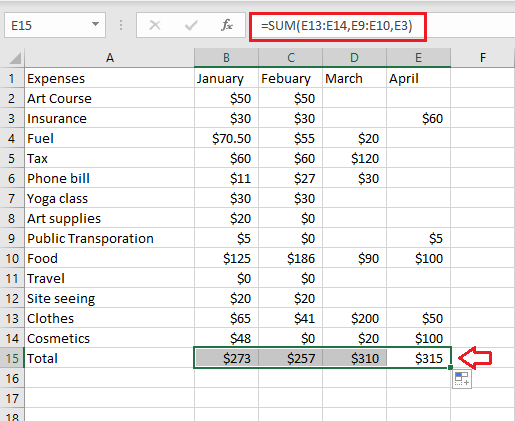
Next, after releasing the mouse, the same formula is placed inside the selected cells and you can see the results.
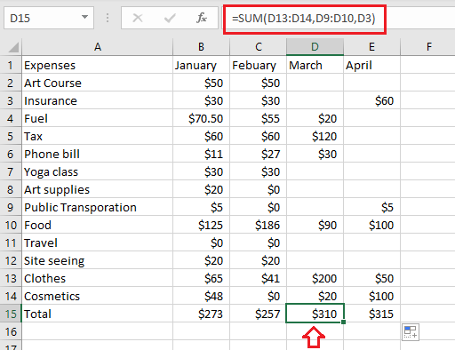
Let’s check the formula of the adjacent cells and compare it with column E; the same formula is reproduced. You can also perform the same for rows.
I hope you found this blog helpful. If you need to know more about other Formulas and Functions, check out our other blog on “How to Calculate Average in Excel” and “How to Subtract in Excel.”
Now that you know how to sum numbers in Excel, you can take your Excel skills to the next level by learning how to subtract in Excel. Read our guide on subtraction here.
To get a better insight on our Excel services check out Microsoft Excel Consulting Team and Excel Support
Our experts will be glad to help you, If this article didn’t answer your questions. ASK NOW
We believe this content can enhance our services. Yet, it’s awaiting comprehensive review. Your suggestions for improvement are invaluable. Kindly report any issue or suggestion using the “Report an issue” button below. We value your input.


