How To Transpose In Excel

There are several ways to rearrange data in Excel. One of these ways is Transposing, which lets you convert rows to columns (or vice versa) easily, instead of typing the data one by one. For example, sometimes, we find out it’s better to switch the columns and rows. So in this tutorial, we’re going to learn how to do this.

There are two quick and easy ways to transpose the data:

1. Paste Special
2. The Transpose Function

The other way, which is not as simple as the two other ways, is using Arrays. If the data is the output of particular software, or if you always receive specific data with a specific format and tabulation, in the form of a table from a source, and you continuously need to transpose them in Excel using array formulas will make it easier. With this method, you will no longer need to perform repetitive operations of transposing with the two methods mentioned above.

Paste Special

To switch rows and columns in Excel  using the Paste Special option, follow these steps:

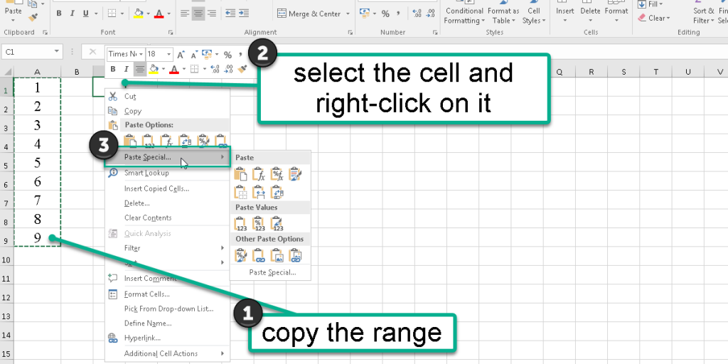
1. Select your data.
2. Copy the range you selected (use the Copy option from the menu by right-clicking on the rang or press Ctrl+C.)
3. Select the cell you want to present the result, right-click and choose the Paste Special option.

 

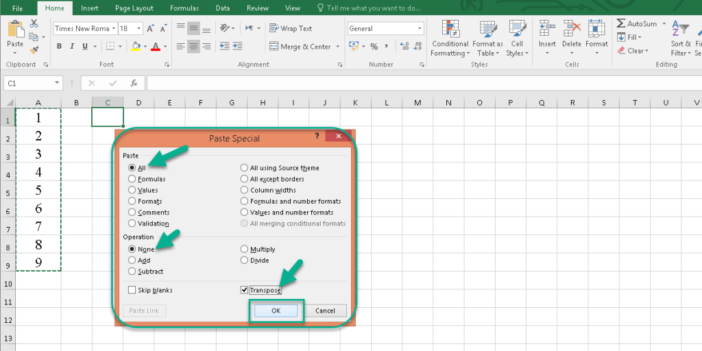
4. From the Paste Special dialogue box, check the Transpose checkbox and press OK.

 

Note: the shortcut of the transpose is the icon. You can find it from the Paste Special menu.

 

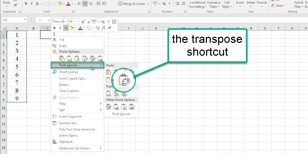
As you see, this is an effortless way to transpose your data and convert the rows to columns and vice versa, using the Paste Special option.

 

 

The Transpose Function

These steps help you transpose your data by the Transpose function:

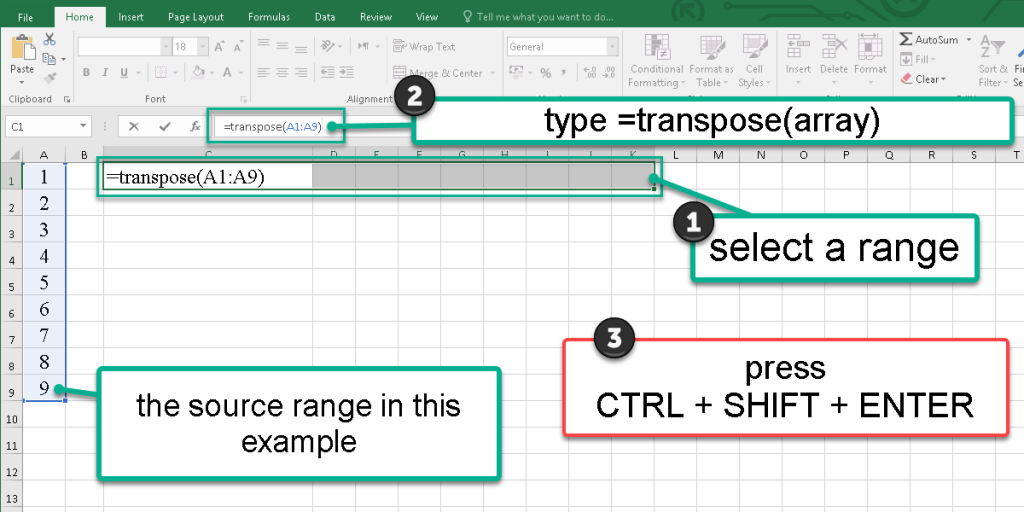
1. Select a range you want to see the result there.
2. Enter =Transpose(array) in the Formula bar (or type the formula in a cell).

Note: The Array argument here is the source range of the data.

3. Press CTRL + SHIFT + ENTER to apply the function as an array to the destination cells.

 

Note: This function is only used when you enter it as an array formula.

 

 

 

Here is an example of how to rotate tables and data in Excel.

Note: when you want to rotate a table, the Paste Special option is disabled. So you should use the second method, which is using the Transpose function.

Example- 

In this example, we have a simple table of random numbers. This table contains three rows and six columns.

Step 1: Select a range that contains six rows and three columns.

Step 2: In the Formula Bar, enter the Transpose function.

=transpose(array)

Step 3: For the Array argument, select the table range (except the headers.)

 

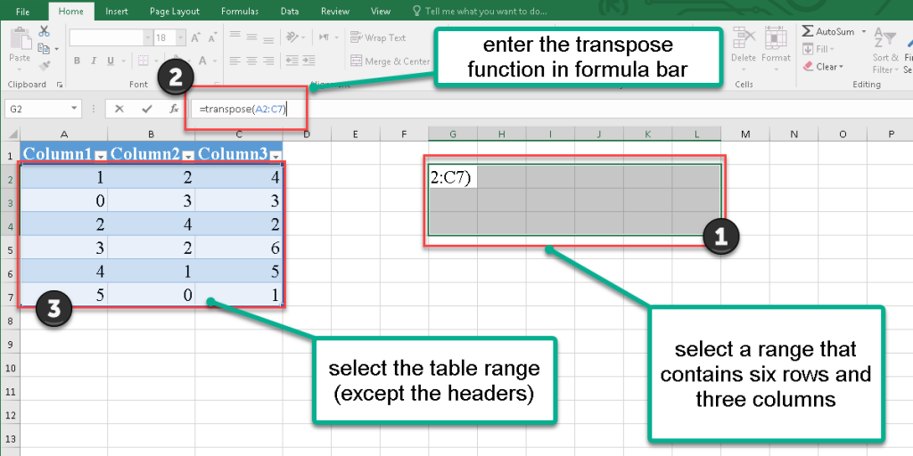
Step 4: Now press Ctrl+Shift+Enter.

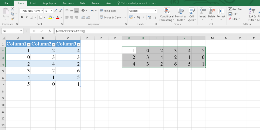
You can see the result in picture 6.

 

You can connect with us and ask our experts for your inquiries and get more Excel Support Services.

Also, reduce costs, accelerate tasks, and improve quality with Excel Automation Services.