8 Math Formulas in Excel Every Beginner Should Know!

8 Beginner Math Formulas In Excel

If you just started working with Excel, you might search for a tutorial that explains everything at once. Especially in the case of formulas. As you know, Excel is a nifty application that can calculate, and compute an extensive amount of data in seconds. When you add a formula, your computer performs a mathematical operation to produce specific values.

These formulas may seem confusing at first, but it gets easier when you learn how to use them. Many people (beginner and professional) use Excel formulas. But, they may not all know what the rules and signs are about.

Excel Formulas and Functions

While using a calculator, you can perform complex calculations as part of a larger computational process. However, when using Excel, you enter the values into the predefined functions and formulas.

For example, when you want to calculate many numbers using a calculator, you have to enter them all at once. In Excel, you only need to add the numbers in the SUM function and get the result in less than seconds.

Excel Math Formulas Application

Most people think that you can only use Excel for businesses. Yet, there are no limitations in using this well-designed software. For example, you can manage your financial plans as a parent or make an organized list of your student’s results as a teacher. So, here is a nice list of what you can do with math formulas in Excel:

• Manage family budget
• Manage apps and calendars
• Create a checklist and track projects
• The financial calculation, loans, debts, etc.
• Create management dashboard
• Manage invoices and receipts

Excel Formula Tips

Before digging into the formulas, it’s necessary to be informed of signs and relevant points within the procedures. So, here are some essential tips that help you as a beginner.

1. Enter Equal Sign =

The most important thing you should notice as a beginner is entering = (the equal sign). The equal sign is used to start the process when you work with any function or formula.

First step: Enter the Equal sign

2. Colorful Addresses

When you enter a formula, define the addresses, and select cells, you see each one appears in a different color. This would help with better readability and quick identification among cells.

3. Colorful Parentheses

Parentheses are critical signs in formulas. You have to use them a couple of times in only one case. For instance, when managing nested or hybrid functions, Excel defines parentheses with a different color for each function.

Attention, colorful parentheses are shown for different functions, and bright addresses are displayed for different ranges.

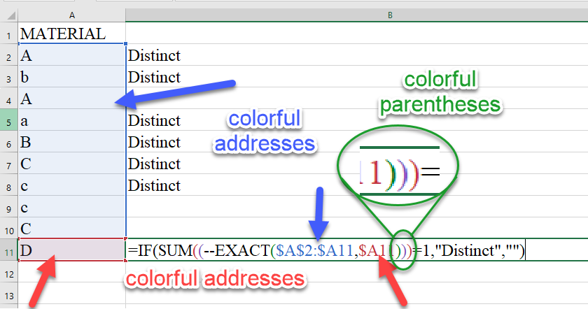
Tip: The first function color is always black. So when the closed parentheses are black, it means no other parentheses should be placed, and you complete the entire formula range.

4. The Brace Sign {}

Before expounding the meaning of a brace, we should learn what an array is.

Arrays in Excel perform calculations themselves and eliminate the need for helper cells. The point is you have to press the Ctrl+Shift+Enter instead of pressing the Enter key. After you press the Ctrl+Shift+Enter and register the array, the entire array formula is placed among braces. 

Every so often, your array formula is a part of another formula. So the point is that braces do not always appear at the beginning of your formula.

5. The Bracket Sign []

When you see a couple of bracket signs in a function guide, you can assume that the statements mentioned among them are optional. Here, optional means that if you don’t enter any value, Excel takes a predefined value depending on the function.

6. Bold Argument

Excel helps you recognize which argument you’re working on by making it bold while adding the values.

 

 

Excel Math Formula

Before getting into the tutorial on the math formulas, let us explain that we start from the most basic ones and work up to the next level. By the way, for each section, a link is provided that explains the section in detail. So you can refer to them and learn more.

Add Numbers, Cells, And Columns in Excel

The most common function in every math calculation is the summation function. Assume you have to sum the values of your data set; there are various ways to add values in Excel. As an introduction to this section, we’ll mention how to add data without formulas or Excel functions; then, we will explain these calculations using formulas and functions.

The Result of Addition on the Status Bar

To catch a glimpse of the summation of the data list without registration, you can follow these steps:

1. Select the data range.
2. Look at the Status Bar that shows the Sum, Average, and Count values.

If the Status Bar doesn’t show these items, right-click on this area and check them. You can also choose other options, such as Minimum, maximum, etc., to be displayed.

Add Values by the Paste Special Option

Here we add numbers of our data set by the Paste Special option. We don’t use any formulas and functions with this option.

Add by Formula in Excel

A simple way to sum values using a formula in Excel is by writing the numbers and inputting the summation sign (+) among them. For instance:

=10+20+30+40+50+60+70+80+90

The problem here is that when you add the data set values one by one like this, you have to change the formula for every change in values because this formula is independent of the cells.

Sum Function

The previous methods we mentioned are not appropriate for large data values. It takes a long time to add hundreds of numbers one by one. So, we make use of the Summation function. Here, we explain how to utilize the Sum function in Excel in several ways?

The AutoSum Option

Excel provides an option that helps sum up the values with only one click. So, to see how it works, follow these steps:

1. Select your data set.
2. Go to the Home tab.
3. From the Editing section, click on the AutoSum button.

As you can see, after you click the Autosum button, the result appears in the bottom cell of your data set.

The Autosum dropdown list helps you calculate the Average, Min, Max, and count numbers. You can use the More Functions button to search for other functions at the end of this dropdown list.

You can also use a shortcut key instead of clicking on the AutoSum button. The AutoSum shortcut key is ALT and +.

Writing the Sum Formula

In some cases, you have to write the formula to do the summation process. For example, your values aren’t in a single sheet, or you need to combine several functions.

To write the Sum formula, follow these steps:

1. Enter the equal sign.
2. Write Sum.
3. Open parenthesis.
4. Select the range or click on the data cells you want to add.
5. Press Enter.

Example:

=SUM(your data range)

Other Ways to Add Values

1. Select a cell, click the fᵪ button and search for the Sum function; press OK, select the range, and press Enter.
2. Select a cell, go to the Formula tab from the Function library, click on the Math and trig button, and choose SUM from the list.

 

 

How to Subtract in Excel

Subtraction in Excel is known to be one of the simple functions. Using the minus symbol, you can easily subtract numbers, cells, columns, and rows in Excel.

We have mentioned five methods in the “How to subtract in Excel” blog, which you can check out. 

The point is that we don’t have any predefined function for this operation in Excel, and we have to do the process manually.

How to Subtract Date and Time

If your data has a Date format, you can subtract the start date from the end date to see the result or use the DATE or DATEVALUE functions. Also, you can use the TIMEVALUE function to convert a time_text into a suitable Excel time.

=TIMEVALUE(time_text)

Example:

Time A: 8:23 PM

Time B: 12:49 AM

=TIMEVALUE(“8:23 PM”)-TIMEVALUE(“12:49 AM”)

How to Subtract Matrix in Excel

If you have matrixes as your data set, you can subtract the data using only one formula.

How to Divide in Excel

As you know, there are many ways to use a function in Excel. The division function is no exception to this rule. You can utilize the Divide function or write it as a formula.

Divide by Formula in Excel

When you divide numbers into a cell, for example, divide 80 into 20, the easiest way is using the divide sign. 

=80/20

Divide a Column into a Number

Sometimes, we need to divide multiple cells into a number. So, keep reading to learn how to do this.

The best way to divide a column into a number is to write the number in a cell and enter the cell address in the formula.

How to Divide by the Paste Special Option

You don’t always need to write a formula to divide numbers; it can be done by copying and pasting.

How to Solve #DIV/0!

Since dividing a number by zero is not defined, Excel shows the #DIV/0! Error. A textual or an empty cell will be given a zero value in mathematical calculations in Excel. So, we prefer Excel to show the open cell instead of a cell that contains an error.

IFERROR Function

By using the IFERROR function, you can solve the #DIV/0! Error. When you write the formula, you can add this function and define a second parameter to represent it instead of the error. 

How to Do Superscript and Subscript in Excel

Working with formulas (especially mathematical, chemical, etc.) needs particular text formats. Excel provides options that help you write these formulas in better ways, including the superscript and subscript. You can use them in both cells and charts.

These features help users understand values and make formulas appear better, such as H₂O, x², x^y+z, etc.

Superscript

A superscript value is smaller than a regular object above the standard line. For instance, x², x^y+z, etc.

Subscript

A subscript value is similar to a superscript but under the standard line, such as H₂O, x₁+x₂, etc. 

How to Do Superscript and Subscript in Excel by Font Option

You can also do subscript and superscript text, numbers, etc., by the Font option in Excel. 

How to Extrapolate in Excel

Forecasting is the most important way of analyzing data. Knowing the  future demand, sales, production, etc. amount helps managers decide brightly and move more accurately. This is where Excel comes into its own.

We intend to introduce extrapolation here; however, you can find a more detailed explanation of each part in the How to extrapolate in Excel blog.

Linear Extrapolation

The Extrapolation formula

You can extrapolate data by the Extrapolation formula. Here, you need two points of a linear chart.

• A(a, b)
• B(c, d)

Y(x)=b+(x-a)*(d-b)/(c-a)

Extrapolate by Trend Line

What’s great about Excel is that it makes this easier for you by the Trend line option. You can extrapolate your data from linear or nonlinear graphs using the Trend Line option. Bear in mind that this option cannot be used for Radar, Pie, Doughnut, Bubble, and 3D charts.

To add a trend line to your chart, click the Chart Element icon and check the Trend line.

We have six trend line types that you could choose based on your data change trend. These six types are:

1. Exponential
2. Linear
3. Logarithmic
4. Polynomial
5. Power
6. Moving Average

Extrapolate by the Forecast Formula

Another handy Excel option is the Forecast option which doesn’t need charts and graphs to forecast data. The Forecast. linear and Forecast.ETS functions are subject to the Forecast function and support your data over a linear trend, periodical templates, and sheets.

The syntax of these functions are:

• The Forecast. linear syntax

=FORECAST.LINEAR(x؛ known Ys؛ known Xs)

• The Forecast.ETS syntax

=FORECAST.ETS (target date؛ values؛ timeline؛ [seasonality], [data_complation]; [aggregation])

Extrapolate sheets

By Extrapolating sheet option, you can see the result of forecasting a sheet such as:

• Where the Forecast starts or ends
• Change the confidence interval
• Add the Forecast statistics
• Change the Timeline and Values range
• And aggregate duplicate using

To create a visual forecast worksheet in Excel 2016 and later versions, go to the Data, and click the Forecast Sheet button to open the Create Forecast worksheet box.

Extrapolate by the Trend Function

One of the statistical functions based on linear regression is the Trend function which predicts future trends without needing graphs.

The syntax of the Trend function is:

=TREND(known_Ys; [known_Xs]; [new_Xs]; [const])

How to Interpolate in Excel

A data set composed of dependent and independent variables shows specific numbers. However, sometimes we need a point between the two points we have. By interpolation, we estimate new data points according to the known range. When it comes to nonlinear functions, we can’t determine the exact place of the point in some cases. Yet, we are able to estimate them.

Here, we’ll mention the methods briefly, but in the “What is Interpolation and how to interpolate in Excel?” blog, the process is explained thoroughly.

Linear Interpolation

Mathematically speaking, Crossing a straight line between the two data points you have, is called Linear Interpolation. You can do this manually by using the equation, but a better choice would be to use these functions to speed up the process.

1. Linear Interpolation by the Trend Line

Plot a chart for your data set and add a trend line. This option gives you an equation to find the value you want (Y) by putting the desired amount (x).

2. SLOPE and INTERCEPT Functions

The SLOPE and INTERCEPT functions are helpful when we don’t want to plot charts and graphs. We need to realize the slope and intercept for linear interpolation to detect a linear function. This is the Trend Line feature base method called linear regression.

The SLOPE and INTERCEPT functions syntax are:

=SLOPE(known_y’s, known_x’s)*x+INTERCEPT(known_y’s, known_x’s)

3. Interpolate by the Forecast Function

Another prediction operation to interpolate linear functions is the FORECAST or FORECAST.LINEAR operation.

The FORECAST syntax is:

=FORECAST.LINEAR(x, known_y’s, known_x’s)

4. Interpolate by the Trend Function

The Trend function could discover an unknown value by the known y’s and x’s values.

The TREND function syntax is:

=TREND(known_y’s,[ known_x’s], [new-x’s], [const])

[const] is a logical argument defined by two values; one or zero. If you suppose it as one, the function calculates the intercept typically, and zero means the intercept will be zero in the calculation.

Nonlinear interpolation

Having a data set with a nonlinear behavior is more common than linear behavior in the real world. So nonlinear interpolation knowledge is typically necessary. However, you should detect your function behavior before you do the interpolation. 

Nonlinear Interpolation Using Trend Line

Using an appropriate trend line based on your data set is the key to interpolating data appropriately. Here, in “Nonlinear Interpolation Using Trendline,” you can follow the steps and learn more about nonlinear interpolation.

Growth Function

With regards to exponential behavior, we have a function that predicts values according to the exponential regression: Y=b*m^x

The GROWTH function syntax is:

=GROWTH(known_y’s,[known_x’s],[new_x’s],[const])

Multiply Cells and Numbers

Multiplying data in Excel is indeed one of the most common functions. So, we’ll attempt to present a few different multiplication methods in this blog.

To multiply numbers in Excel, you can use the multiplication sign *. For instance, A1*B1, 2*3, A1*5, etc., but continue reading to see the Multiplication function and how we generally use it. 

As a matter of fact, we have discussed multiplication fully in the “How to Multiply in Excel” blog.

Note: When you use multiple operators to write a formula, observe the computational priority of these operators. Consider the acronym term PEMDAS for this purpose.

1. Parentheses
2. Exponentiation
3. Multiply and Division
4. Addition and Subtraction

Multiplication Function

The multiplication function in Excel is defined as the PRODUCT function. You can use the PRODUCT function to multiply two or more numbers, cells, or even multiple ranges of data.

=PRODUCT(number1, [number2], …)

Multiplication by the Paste Special

Doing multiplication without using formulas or functions could be done by the Paste Special option in Excel. But the point is that dependent cells will not form since you did not use any formula to perform the multiplication operation in this method. This means that the multiplication result will not change by changing cells.

SUMPRODUCT and IMPPRODUCT

The SUMPRODUCT is a function that calculates the summation of the product results. 

How to Multiply Complex Numbers in Excel

To do engineering calculations in Excel, we use complex numbers. These calculations are often different from how we calculate Real numbers, such as multiplying complex data by the IMPRODUCT function.

How to multiply matrices

If you have already multiplied two matrices, you know that these calculations are too long. Here, Excel does the multiplication quickly and displays the result immediately by the MMULT function.

How to Round Numbers in Excel?

Rounding decimal numbers could be done quickly by Excel. Still, many people have problems when working with decimals, such as miscalculations; we have tried to go through them entirely and accurately step by step in the “How to Round Numbers in Excel” blog.

Here, we’ll take a brief look at how to round numbers?

We have two general methods to round numbers in Excel:

1. Manually
2. Using Functions

Round-Off

Rounding off values means changing the numbers’ decimal digits. Excel rounds up or down based on the decimal digits to 5. For example, 3.2 will be rounded down to number 3 (2<5), and 3.6 will be rounded up to number 4 (6>5).

The manual way to round numbers is using the Increase and decrease decimal options in the Number section of the Home tab.

To round numbers using a function, you can write this syntax:

 =ROUND(number, num_digits)

Round-Up & Round-Down in Excel

Rounding up is a specific part of the rounding process, and it turns the decimal number to the next number, such as:

=ROUNDUP(153.6, 0) = 154

 =ROUNDUP (506.9543, 3) = 605.955.

The Round-Up function Syntax is:

=ROUNDUP(number, num_digits)

The Round Down function is similar to the Roundup, but it turns the number to the previous number. For example, the result of =ROUNDDOWN (1.1111, 1) would be 1.1, or =ROUNDUP(6.92156, 0) would be 6.

The Round-Down function Syntax is:

=ROUNDDown(number, num_digits)

Rounding Based on Coefficient in Excel

Note:  The Coefficient means that if a number is divisible by a Multiple argument number, the remainder must be zero.

We have seven rounding formulas in Excel that round numbers based on a coefficient. Previously, we mentioned what these seven formulas were and how to use them, we are now going to explain a few arguments.

1. Multiple: Multiplier we use for rounding.
2. Significance: The number we want to round the first argument’s value to a multiple of. The default for this argument is 1.

3. Mode: Round negative numbers to zero or farther from zero whose default number is zero.
   1. If the mode is zero (or does not mention), negative numbers are rounded to zero.
   2. If the numeric mode is zero, the negative numbers are rounded away from zero.

Bottom line

One of the most powerful features in Excel 2010 and later versions is calculating practical information using formulas. Like a calculator, Excel can add, subtract, multiply or divide.

There is almost nothing Microsoft Excel can’t do for computing, from adding a column of numbers to solving complex linear programming problems. You can connect with us, ask our experts if you have any inquiries, and get more support via Excel Support Services.

Also, reduce costs, accelerate tasks, and improve quality with Excel Automation Services.

FAQ: